Dynamic displacement monitoring of flexural structures with distributed long-gage macro-strain sensors

Abstract

A new method is proposed to monitor dynamic displacement for flexural structures especially. In this method, the distributed macro-strain is first obtained using long-gage fiber Bragg grating sensors. Then, the conjugated beam theory is applied to calculate the displacement. To verify the method, a cantilever beam, installed with the proposed sensors, is subjected to free vibrations. The results from the proposed method agree well with those measured by the traditional displacement transducer as the error for the first three peak values is less than 5%. A finite element model of a simply supported multi-girder bridge is also simulated with a truck load. The results show that the proposed method can evaluate dynamic displacement accurately as the error for the maximum displacement is less than 3% in all the cases. Finally, the method is verified using simply supported beam models subjected to random dynamic loads. However, the sensor gage length shows some influence on the results. To ensure exact measurements, the sensor gage length should be limited to be smaller than 1/20 of the beam length. Considering other advantages of fiber optic sensing, the proposed method shows promise in the field of long-term structural health monitoring.

Introduction

Flexural structures such as those involving beams are the most common components of civil infrastructure today, especially in bridges. However, factors such as overloading, original structural flaws, and typhoons jeopardize the safety of these structures and have attracted attention from the public. Structural health monitoring (SHM) was proposed and applied as a solution to ensure structural safety.^1–3

Displacement is a key parameter in the design process of flexural structures such as classical girder bridges and is usually required for monitoring with SHM. Due to dynamic effects, the dynamic displacement is of greater importance in evaluating structural performance than the static displacement. However, it is difficult to accurately obtain dynamic displacement values, especially for long-term on-line monitoring.

Measuring displacement with displacement transducers, such as linear variable differential transformers (LVDTs) or dial gages, is simple during laboratory testing. However, field tests on existing structures require additional scaffolding to support the displacement transducers, and such issues cannot satisfy the needs of long-term SHM. To solve this problem, Carlos et al. ⁴ developed a novel displacement transducer to measure vertical bridge deflections based on fiber optic fiber Bragg grating (FBG) sensors and a non-contact measurement technique supported by a liquid leveling system. However, this system may not implement dynamic monitoring accurately because the liquid system’s lag is too great. The global positioning system (GPS) has become the method used for this type of monitoring over the last two decades, especially for the SHM of large-scale bridges. Nakamura ⁵ presented an example using a kinematic GPS with a low sampling rate to monitor suspension bridge displacement. Lovse et al. ⁶ illustrated an example of how a GPS could be used to monitor the dynamic deflection of the Calgary Tower in Canada. To improve the performance of GPS, Gethin et al. ⁷ proposed a new system involving the hybrid use of GPS and accelerometers. However, GPS is limited by multi-path and cycle slips, a relatively low frequency of data, and the need for good satellite coverage. A technique involving lasers is also popular. Hani et al. ⁸ accurately determined the dynamic deflections of bridges under live traffic loads using a non-contact laser Doppler vibrometer (LDV) system. Hyun et al. ⁹ proposed a multiple paired structured light system as a displacement measurement system and illustrated the feasibility of the system for long-span structural displacement measurement. However, these types of laser sensors may not suitable for long-term SHM because they are often placed on the ground underneath the bridge and cannot be left unattended. Many other interesting proposals have also been implemented, such as photogrammetric deflection measurements ¹⁰ and radar-based displacement sensors. ¹¹

As stated above, these methods are applied to measure displacement directly to some extent. Some indirect methods were also studied and implemented for measurement using other physical quantities mathematically related to displacement.^12,13 These methods were considered an important solution for extracting dynamic displacements by double integrating the measured acceleration data. ¹⁴ However, the low-frequency error from the limited low-frequency response capability of accelerometers was easily amplified during the numerical integration of the digital acceleration data. Strain is another parameter often used to assess displacement. Tommy et al. ¹⁵ used a polynomial equation to evaluate the vertical displacement of bridges with the strain measurements from FBG sensors. Major errors can occur due to the style of such a “point” sensor installation, especially under random complex loads. Baz and Poh, ¹⁶ Li and Ulsoy, ¹⁷ and Wang et al. ¹⁸ introduced a method for extracting dynamic displacement from strain based on modal analysis. It was a really good method to obtain the displacement just with several strain sensors. However, it was difficult to accurately obtain the mass-based normalized matrix of strain and displacement modes during field testing. Cho et al. ¹⁹ proposed an improved method to get a relatively accurate mode shape using finite element (FE) model. However, the problem still needs to be solved further. To solve the problem, Xia et al. ²⁰ proposed an efficient method for bending beam type structures to get the dynamic displacement from several strain sensors. In their method, the rotation angle was first obtained from the measured strain and then the dynamic displacement was calculated with the rotation angles. The proposed method was applied to the 600-m-tall Canton Tower and found a good agreement with the measurements using GPS and inclinometers. However, there is some risk which may decrease the effects. If some of the strain sensors are influenced by the local concrete cracks, the displacement may be overestimated. Bassam and Ansari ²¹ introduced another method using the matrix of shape function to obtain the lateral displacement from the measured element strains and verified with experiments. It seems to be an effective way to monitor the dynamic displacement from the strain measurement.

This article proposes a new method based on the distributed macro-strain sensing technique and classical conjugated beam theory to monitor dynamic displacement, especially that of flexural structures. The proposed method obtains the distributed macro-strain–time history using long-gage FBG sensors and then extracts the dynamic displacement from the measured strain using conjugated beam theory. Finally, the performance of the method is verified with vibration tests on a cantilever beam and FE models of a classical simply supported multi-girder steel stringer bridge, and a simply supported beam.

Distributed macro-strain measurements using long-gage sensors

Distributed long-gage macro-strain sensors

FBG sensors have attracted attention for their use in SHM due to their excellent accuracy, high data acquisition speed, and multiplexing performance. Based on the FBG technique, a long-gage macro-strain sensor is developed at every point in the gage length with identical mechanical behavior, and hence, the strain transferred from a shift of the Bragg center wavelength represents the average strain over the gage length, named as macro-strain. To make the long-gage concept useful in real sensors, the FBG sensor is fixed at two ends within a tube made of plastic material but having elastic characteristics surrounded by a fiber sheath that is impregnated with epoxy resin. Figure 1(a) shows the schematic of the long-gage FBG sensor. The diameter of the packaged sensor is approximately 2 mm, as shown in Figure 1(b). The gage length can be set from 0.1 to 1 m.

Figure 1.

Packaged long-gage FBG sensor: (a) schematic diagram and (b) actual sensor.

The greatest advantage of this long-gage FBG sensor is that it provides an efficient way to realize distributed sensing. The proposed long-gage FBG sensors are connected to each other to cover the study area of the structure, as shown in Figure 2. Moreover, compared with the bare FBG, there are some obvious ad advantages as follow: (1) it is strong enough to survive the harsh civil engineering environment as package material, fiber, is of high strength; (2) the package will greatly decrease the effects from outside substance, such as water and sunlight, on the optic fiber sensor.

Figure 2.

Distributed macro-strain measurement with long-gage sensors.

Distributed macro-strain measurements

A cantilever beam was selected to verify the strain sensing performance of the proposed long-gage sensors. The beam was made of a fiber-reinforced polymer (FRP) board, with a length of 800 mm, width of 155 mm, and depth of 7 mm. Three types of sensors were applied for comparison: the bare FBG, packaged FBG, and common strain gage. The gage length was 150 mm for all bare and packaged FBG sensors, while the strain gages were installed at the midpoint of each monitored element. Detailed information on the sensor distribution is shown in Figure 3. With this style of sensor distribution, the strain values were expected to be same for all three sensors on an identical monitored element.

Figure 3.

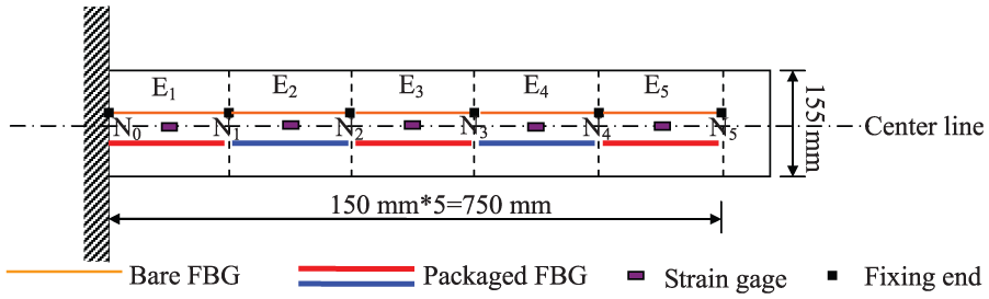
Sensor distribution on the tested cantilever beam (view from above).

Static and dynamic tests were performed to evaluate the sensing performance of the proposed long-gage sensors. The static load was loaded at node N₅, while the free vibration was applied through a preset displacement of about 5 mm at the free end of the beam. The sampling speed of the dynamic tests was 1000 Hz.

The results of static tests are presented in Figure 4 to illustrate the distributed sensing and evaluate the measurement accuracy. The original strain results are shown in Figure 4(a), in which the values measured from the packaged FBG are obviously larger than those from the other two types of sensors. Sensor size was the main reason for this difference. The radius of the packaged FBG was approximately 1 mm, while the depth of the beam was only 7 mm. Therefore, the distance from the installed packaged FBG to the neutral axis was approximately 4.5 mm. However, the other two sensor types were so small that the distance from the sensor to the neutral axis was only 3.5 mm. Basic beam theory explains why the values measured from the packaged FBG were larger. The results were subsequently modified to consider the sensor sizes, as shown in Figure 4(b), after which the results from the three sensor types were close to each other for every element, and the largest standard deviation was only 2 µε. Meanwhile, the strain distribution showed excellent linearity along the beam. The correlation coefficient of the linear fitting was larger than 0.99, which was in accordance with the theoretical analysis.

Figure 4.

Static strain distribution: (a) original data and (b) modified to consider sensor size.

Some dynamic strain results are given as examples in Figure 5 to illustrate the performance of the dynamic strain sensing technique. In this case, all of the results of the packaged FBG were modified to account for sensor size. The figures show close values of all the sensors. However, the results of the strain gage display obvious noise, which is less noticeable for the FBG sensor.

Figure 5.

Dynamic measurement: (a) E₁ and (b) E₃.

Theory of extracting displacement from strain sensing

The classical conjugated beam method was first presented by Breslau in 1865. Theoretically, a change in load form or its value is equivalent to a change in the bending moment distribution along the axis of a beam. According to the method, the absolute values of curvature distribution in the original beam are equal to the absolute values of load distribution in the conjugated beam. Then, the bending moment distribution of the conjugated beam under the equivalent load distribution is equal to the value of the displacement distribution of the original beam. In other words, the displacement can be extracted only with the strain distribution and neutral axis distribution. Compared with the double integration method, the obvious advantages of this method are that the section bending stiffness EI is not needed and less error can be expected with one integration. In this article, the method is proposed about so-called Bernoulli’s beam.

The distributed strain measurement should be implemented with this method for monitoring, especially under arbitrary load conditions. The distributed macro-strain measurement based on long-gage sensors is an appropriate and actual choice. Based on the proposed distributed strain sensing style, the extraction of displacement from strain is illustrated with the conjugated beam method. This study uses the classical cantilever beam and simply supported beam as examples.

In Figure 6(b), the load q_i can be expressed as

$$q_i=\frac{M_i}{{(\mathrm{EI})}_i}=\frac{{\epsilon }_i}{y_i}$$

(1)

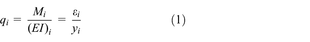
where M_i, (EI)_i, ε_i, and y_i are the average moment, average section stiffness, macro-strain, and average distance from the sensor to neutral axis for the ith monitored element of the original beam as shown in Figure 6(a), respectively. For dynamic monitoring, equation (1) can be written as equation (2) at time t

$$q_i(t)=\frac{{\epsilon }_i(t)}{y_i}$$

(2)

Figure 6.

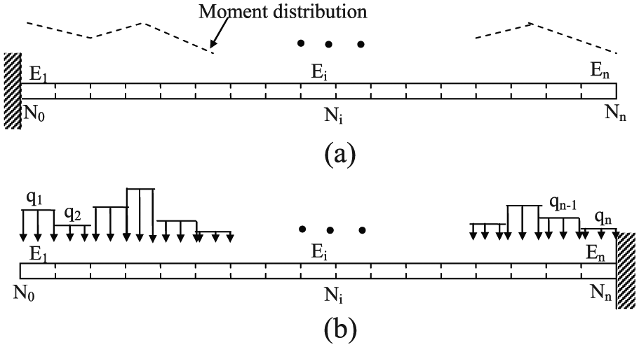
Cantilever beam model: (a) original beam and (b) conjugated beam.

Then, the dynamic displacement at node N_i for the cantilever beam is

$$\begin{array}{l}{D}_i(t)={\displaystyle \sum _{j=0}^i{q}_j(t)}\times l\times (i-j+0.5)\times l\\ ={\displaystyle \sum _{j=0}^i\frac{{\epsilon }_j(t)}{y_j}}\times (i-j+0.5)\times l^2\end{array}$$

(3)

Here, the element length is assumed to have a uniform value l for all elements. q₀ is set to zero.

Similarly, the dynamic displacement at node N_i for the simply supported beam shown in Figure 7 can be expressed as

$$\begin{array}{c}\multicolumn{1}{c}{D_i=[\sum _{j=1}^n{q}_j(t)\times l\times (n-j+0.5)\times l]}\\ \times \frac{1}{n\times l}\times i\times l-\sum _{j=0}^i{q}_j(t)\times l\times (i-j+0.5)\times l\hfill \\ =\sum _{j=1}^n\frac{{\epsilon }_j(t)\times (n-j+0.5)\times l^2\times i}{y_j\times n}\hfill \\ -\sum _{j=0}^i\frac{{\epsilon }_j(t)}{y_j}\times (i-j+0.5)\times l^2\hfill \end{array}$$

(4)

Figure 7.

Simply supported beam model: (a) original beam and (b) conjugated beam.

The displacement at node N₀ is not included in equation (4), so D₀ is set to zero due to the support constraints.

Verification with a cantilever beam

Experimental setup and sensor installation

To verify the performance of the method described in section “Theory of extracting displacement from strain sensing,” a cantilever beam was applied to complete certain dynamic tests using the distributed long-gage macro-strain sensors. In Figure 3, the prepared beam is shown installed with three types of strain sensors, namely, bare and packaged FBGs and strain gages, which number is 15 in total. The gage length was 150 mm for the two types of FBG sensors. In other words, the strain extracted from the sensor indicated the average value over 150 mm of the beam. Other descriptions of this scenario can be found in the first paragraph in section “Distributed macro-strain measurements.” For comparison, a displacement transducer was installed at node N₅ to obtain the true displacement value, as shown in Figure 8. Three different displacement values, about 10, 15, and 20 mm, were preset at node N₅ to cause free vibration, and the cases were named Case I, Case II, and Case III, designed to simulate small, medium, and large deformations, respectively. The speed of data acquisition was 1000 Hz for all the sensors.

Figure 8.

Displacement transducer on the tested cantilever beam (view from the side).

Results and analysis

Dynamic strain was obtained first. In Figure 9, the strain–time history of E₁ is given as an example to illustrate the strain measurement accuracy. The results of the packaged FBG were modified to consider sensor size, and this modified strain was used to calculate the displacement. As discussed in section “Distributed macro-strain measurements,” the sensors displayed similar trends and close values, except for some obvious errors arising in the strain gage. The standard deviation between the strain gage and FBG was approximately 12 µε, whereas it was only 3 µε between the two FBG sensor types.

Figure 9.

Dynamic strain measurement of E₁: (a) Case I, (b) Case II, and (c) Case III.

The dynamic displacement was obtained using the measured distributed strain in equation (3). Therefore, the displacement–time history from nodes N₀ to N₅ was easily obtained. However, only the results at node N₅ were included in this article to illustrate the efficiency of the proposed method and are shown in Figures 10–12. Figures 10(a), 11(a), and 12(a) indicate that the results from the four sensor types gave the same vibrations over the entire time history. Partial time histories were selected to assess the results in detail, as shown in Figures 10(b), 11(b), and 12(b), especially from the first three peak values. It became clear that the measurements from the FBG sensors were close to those of the displacement transducer, which were considered the true values because their relative errors were below 5%. The accuracy was not affected by the different cases. However, the accuracy of the strain gage was not as high as that of the FBG sensors as the noise is obvious. Indeed, the noise could be decreased with noise filtering methods. However, compared with the FBG sensor, the strain gage was found to actually be a disadvantage, especially in long-term monitoring.

Figure 10.

Dynamic displacement measurement at N₅ for Case I: (a) entire time history and (b) partial time history.

Figure 11.

Dynamic displacement measurement at N₅ for Case II: (a) entire time history and (b) partial time history.

Figure 12.

Dynamic displacement measurement at N₅ for Case III: (a) entire time history and (b) partial time history.

Verification with a bridge model

Model description

A FE model of a classical simply supported bridge was constructed to assess the effectiveness of the proposed method through a more intensive study. The investigated bridge was a composite of still and concrete that was simply supported with pin and rocker bearings. The deck of the bridge was cast using stay-in-place forms and the bridge also contained typical steel wind braces and diaphragms. In the FE model, the flange thickness was designed to be constant across the 36-m span and full integration between the steel girders and concrete deck was supposed. The neutral axis position was a key parameter in this method in addition to strain distribution. Thus, a solid element was selected to construct the girders and deck, and the parameters could be extracted only with dynamic measurements. More detailed information can be found in Figures 13 and 14.

Figure 13.

FE bridge model.

Figure 14.

Load distribution: (a) direction of movement and (b) cross section of the bridge.

The traffic load, a truck, was simulated to implement the dynamic measurement. In Figure 14(a), two concentrated loads indicate the loads from the two truck axles. The distance between the two loads was 3.5 m, while their values were both set to 50 kN. The truck was considered to be driven in Lane 2, so the loads were set on the centerline of Lane 2. Four different speeds were designed to verify the method: 36, 72, 108, and 144 km/h; these were named Case I, Case II, Case III, and Case IV, respectively.

Results and analysis

The nodal displacement was extracted first, after which the distributed macro-strain was calculated. Only displacement in the z-direction was applied to extract the strain. Because it had the largest deformation response, the results from Girder #4 were used as examples to verify the proposed method.

Figure 15 presents the typical strain–time history of all the elements in Case II as an example. These strains occurred at the bottom of Girder #4, and the gage length of these macro-strains was 1 m. There were some abnormal negative strains in the first four elements, which may have occurred due to the combination of the end constraints in the z-direction near these elements and the effects of torsion. However, the results of most of the elements were still satisfactory.

Figure 15.

Typical strain–time history of all the elements in Case II.

Using equation (4), the displacement in the y-direction was calculated with the obtained distributed macro-strains. The distance from the neutral axis to the girder bottom was 1.116 m for the extracting process which was included in another paper prepared by the author. Figure 16 shows the results at the mid-span of Girder #4 for all four cases. The theoretical value of the dynamic displacement in the figures was obtained directly from the FE simulation. The calculated values in the four cases were close to their theoretical counterparts, even though some small errors existed. The largest relative error for the maximum displacement was less than 3%, and there was no obvious relationship between error and speed. Thus, the proposed method is proved to monitor dynamic displacement accurately.

Figure 16.

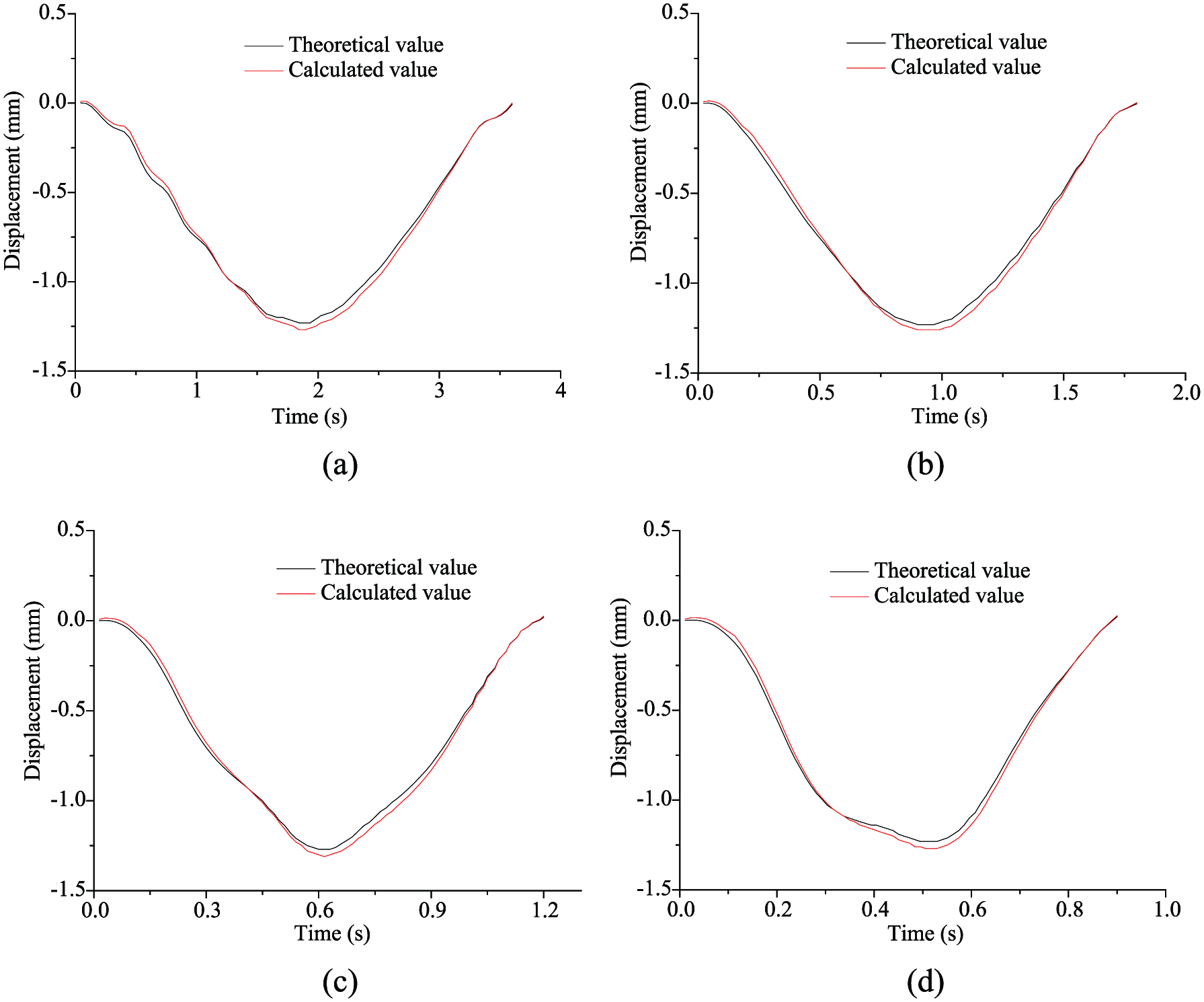
Displacement results: (a) Case I, (b) Case II, (c) Case III, and (d) Case IV.

Verification with a beam model under complex dynamic loads

Model description

When considering traffic loads, the static weight makes up a large component of the total dynamic load. Therefore, the analysis in section “Verification with a bridge model” can be considered a static analysis. To evaluate the performance of the proposed method under complex dynamic loads, a simply supported beam was constructed using FE with multi-point excitation. Nine excited points were distributed evenly along the beam, as shown in Figure 17. A span of random dynamic loads was loaded at each point for 2 s with a sampling rate of 100 Hz. The input random excitation was simulated by white noise, parts of which are shown in Figure 18(a).

Figure 17.

Beam model and loading positions.

Figure 18.

Typical loading and displacement distribution: (a) dynamic loads and (b) displacement distribution.

The beam is 10 m long with a cross section measuring 0.2 m × 0.4 m, and the beam elements were implemented into the simulation in 0.1 m increments, for 100 total elements. The elemental strain was easily extracted after loading, after which the dynamic displacement was calculated with equation (4). Different sensor gage lengths of 0.1, 0.2, 0.5, and 1 m were applied to investigate their effect. Taking the gage length of 0.5 m as an example, the sensor number was 20 for the distributed sensing. Each sensor covered five elements of the beam. In other words, the strain obtained from the sensor represented the average value of the five covered elements.

Some other considerations were also addressed in this study. The elastic modulus was changed to make Model 1 as a “stiff” beam of a first bending mode frequency of 9 Hz, while Model 2 as a “soft” beam of a first bending mode frequency of 0.1 Hz. The typical displacement distribution shown in Figure 18(b) made it clear that the vibration of Model 2 was more complex than that of Model 1.

Results and analysis

After the elemental strain was extracted, the macro-strain was obtained for each gage. Then, the nodal displacement was calculated using the distributed macro-strains. As before, the theoretical nodal displacement was extracted directly from the FE results. To verify the proposed method, Figures 19 and 20 present the displacement results at the mid-spans of the two models.

Figure 19.

Displacement results at the mid-span of Model 1 for different monitoring gage lengths: (a) 0.1 m, (b) 0.2 m, (c) 0.5 m, and (d) 1 m.

Figure 20.

Displacement results at the mid-span of Model 2 with different monitoring gage lengths: (a) 0.1 m, (b) 0.2 m, (c) 0.5 m, and (d) 1 m.

The gage length of Model 1 in Figure 19 had no obvious effects on the accuracy of the method, even when the sensor gage length measured up to 1 m, or 1/10 of the beam length. Upon more detailed study, the absolute values of the relative errors at the peaks were approximately 0.09%, 0.12%, 0.29%, and 0.92% for the four sensor gage lengths, 0.1, 0.2, 0.5, and 1 m, respectively. Although the error became larger with an increase in gage length, this effect was ignored because the error value remained smaller than 1%.

The results of Model 2 in Figure 20 were quite different. The absolute values of the relative errors at their peaks were approximately 1.5%, 2.9%, 5.8%, and 27.5% for the four sensor gage lengths. Here, the sensor gage length had a major effect on accuracy when the vibration contained high-order modes. Therefore, it was concluded that the sensor gage length should be limited for accurate measurement. The results from Model 2 suggested that the sensor gage length should be smaller than 1/20 of the beam length.

Conclusion and remarks

This article presented a new method for monitoring dynamic displacement. The classical conjugated beam theory was employed as the theoretical basis, while the proposed distributed long-gage macro-strain sensors formed the objective basis. The dynamic displacement of flexural structures was properly monitored with the appropriate combination of these elements. Therefore, the following conclusions were drawn based on the illustrations and verifications in this article:

1. The proposed distributed long-gage macro-strain sensors could be applied to evaluate precise dynamic displacements during the structural monitoring of common beams because the illustrated errors from the cantilever beam tests and FE simulation were smaller than 5%.

2. The sensor gage length had to measure less than 1/20 of the beam length to accurately monitor beams with complex vibrations, such as those in large-scale suspended bridges.

3. Combined with the advantages of fiber optic sensing, this system showed promise in future long-term SHM.

There are some inevitable limits to the research performed in this study. For example, in the proposed method, the packaged FBG sensors should be installed along the whole structure making a high cost which may hamper the use of presented approach in real cases. There will be two ways to solve this problem. One is to enlarge the sensing gage of the sensor, such as a gage length of 10 m. Then, a bridge of 500 m only needs 50 sensors to apply the proposed method. The other one is to install the sensors at all the key parts where large strain often occurs, while the strain will be estimated at the location where the sensors are not installed based on measured strain at the key parts. The actual effects of the proposed two ways should be studied and verified. For another example, only the deformations due to strain are included in conjugated beam theory. The movement of supports can also cause dynamic displacement along a beam, but there was nearly no strain in the structures tested, especially the simply supported beam. Future research should modify this method to consider these factors. Moreover, it remains to be seen whether the accuracy exhibited in these tests is sustained in field testing. In conclusion, more research must be performed to make the proposed method more useful and applicable.