
Abstract
Most traditional scheduling problems prioritize optimizing production efficiency, cost, and quality. However, with gradually increasing energy consumption and environmental pollution, the novel “energy-efficient scheduling” model has received increasing attention from scholars and engineers. This scheduling model focuses on reducing workshop energy consumption and environmental pollution and has become a hot topic in the scheduling area. This article proposes a new energy-efficient scheduling mathematical model considering productivity, energy efficiency, and noise reduction with flexible spindle speed for the job shop environment. This model considers the machining spindle speed that impacts the production time, power, and noise to be flexible and an independent decision-making variable. In addition, the evaluation methods of productivity, energy consumption, and noise are presented in this model. To cleanly solve this mixed integer programming model, an effective multi-objective genetic algorithm based on simplex lattice design is proposed. The corresponding encoding/decoding method, fitness function, and crossover/mutation operators are designed based on the features of this problem. To evaluate the performance of this method, three instances with different scales have been designed. The results demonstrate the effectiveness of the proposed model for the energy-efficient job shop scheduling problem.
Keywords
Introduction
Currently, environmental and energy problems have become worldwide concerns that receive increasing attention from most countries. In the future, energy consumption will continue to increase with worldwide development. For example, in 2040, China and India will consume twice as much energy as they did in 2013, as shown in Figure 1 (Energy Information Administration (EIA), 2013). 1 Along with increasing energy consumption, environmental problems are becoming increasingly severe. Therefore, how to effectively reduce carbon emissions and energy consumption has become a hot topic for research. Since the beginning of the industrial revolution, industry has consumed significant energy for production. Manufacturing enterprises are responsible for approximately one-half of the total global energy consumption, 38% of CO2 emissions, and significant pollution.2,3 Therefore, manufacturing enterprises urgently need sustainable development to achieve economic, ecological, and social goals.4,5

Energy consumption in China, USA, and India for 1990–2040 (EIA, 2013).
A manufacturing system is an input–output system that converts energy and material resources into final products, and scheduling is one of the most important sub-systems in a manufacturing system. Taking the process plans of jobs as inputs, the scheduling task schedules the operations of all the jobs on machines while satisfying precedence relationships in the process plans. Scheduling is the link between the two production steps, which are the preparation processes and implementation processes. Traditional studies focus more on productivity and cost and rarely address other aspects, particularly environmental issues. However, Gutowski et al.6,7 noted that more than 85% of the energy consumed was not directly used for actual processing. This finding implies that efforts to improve energy efficiency that focus solely on the machines or processes may overlook a significant energy saving opportunity. 8 In fact, scheduling can significantly impact the energy consumption of the entire manufacturing system. Therefore, reasonable scheduling plans are not only able to improve productivity but also can reduce energy consumption and emissions.2,9,10 In addition, compared to other methods including redesigning machines or processes, shop floor scheduling and plant operation strategies require very little capital investment and can easily be applied to the existing systems.11,12 Currently, with increasing energy consumption and environmental pollution, a novel “low-carbon scheduling” model has become a hot topic for scheduling.13,14
Recently, there has been an upswing in studies on low-carbon scheduling. 2 For the single-machine scheduling environment, Mouzon et al. 3 proposed a multi-objective mathematical programming model and several algorithms for a single computer numeric control (CNC) machine scheduling problem considering the goals of reducing energy consumption and total completion time. Mouzon and Yildirim 13 applied a greedy randomized adaptive search algorithm to a single-machine multi-objective optimization scheduling problem with the objective of minimizing both the total energy consumption and total tardiness. Rager et al. 15 proposed an evolutionary algorithm for energy-oriented parallel machine scheduling. For the flow shop scheduling environment, Fang et al.16,17 presented several new mathematical programming models of the flow shop scheduling problem that consider peak power load, energy consumption, and the associated carbon footprint in addition to cycle time. Bruzzone et al. 18 proposed an approach that relied on a mixed integer programming model in which the reference schedule was modified to account for energy consumption without changing the jobs’ assignment and sequencing provided by the reference schedule generated by an advanced planning and scheduling (APS) system. Dai et al. 19 proposed an energy-efficient model for flexible flow shop scheduling and developed a genetic-simulated annealing algorithm to solve this problem. Luo et al. 20 proposed a new ant colony optimization meta-heuristic considering production efficiency as well as electric power cost for a hybrid flow shop scheduling problem. Keller et al. 21 developed a heuristic method for the hybrid flow shop scheduling problem considering energy flexibility. For the job shop scheduling environment, Liu et al. 8 developed a multi-objective scheduling method for the classical job shop scheduling problem (JSP) considering total energy consumption and total weighted tardiness as objectives. Wang et al., 22 Lu et al., 23 and Yin et al. 24 proposed scheduling model focused on reducing energy consumption and environmental pollution at the workshop level, and they developed some new algorithms to solve these problems.
Based on the above review, current studies on the energy-efficient JSP are lacking. Most of the current energy-efficient scheduling studies focus on single machine or flow shop. 8 However, job shop scheduling is a very important workshop type in the discrete manufacturing industry. All these manufacturing workshops urgently need new methods for sustainable development on the system level. Studies on the low-carbon JSP have only recently begun, and many research topics thus remain unexplored. The motivation of this article has two aspects: from the academic perspective, the models and methods of the energy-efficient JSP have not yet been studied well, and from the application perspective, most workshops in the discrete manufacturing industry use the job shop model. In this article, a new energy-efficient scheduling mathematical model considering productivity, energy efficiency, and noise reduction with flexible spindle speed is proposed for the job shop environment. This model considers the machining spindle speed that impacts production time, power, and noise to be flexible and an independent decision-making variable. This model presents the evaluation methods of productivity, energy consumption, and noise. To effectively solve this mixed integer programming model, an effective multi-objective genetic algorithm (MOGA) based on simplex lattice design is proposed. The corresponding encoding/decoding method, fitness function, and crossover/mutation operators are designed according to the features of this problem. Thus, this article can be used in the job shop environment and may significantly reduce energy consumption and noise emission while increasing productivity.
The reminder of this article is organized as follows. Problem formulation is discussed in section “Problem formulation.” A novel multi-objective algorithm for the energy-efficient JSP is proposed in section “MOGA based on a simplex lattice design for low-carbon JSP.” Experimental studies and discussions are reported in section “Experimental studies and discussion.” Section “Conclusion and future studies” offers the conclusion and proposes future studies.
Problem formulation
This article selects productivity, energy consumption, and noise emission as the three low-carbon scheduling optimization objectives. First, the evaluation models for these three objectives are proposed. Then, the mixed integer programming model of the low-carbon JSP is presented based on the above evaluation models.
This article mainly concentrates on the energy-efficient JSP, which considers three objectives. The main aim of this work is to search an optimal schedule from all feasible schedules. The existing research denoted that spindle speed can be viewed as a main factor that can evaluate energy consumption and noise sound. It can reflect relative difference between different schedules on objectives including energy consumption and noise sound. Therefore, objectives are simplified when constructing mathematical model for this energy-efficient JSP. Meanwhile, recent research also shows that energy consumption and noise sound are related to machine process. However, the most existing methods are based on experience or experiments, which is unsuitable for most practical environment and it is not key point of this article.
Evaluation models of productivity, energy consumption, and noise emission
The normal indicators relative to productivity in the workshop scheduling problem include makespan, total flow time, and average/maximum tardiness. The makespan is the most popular indicator and is used to evaluate productivity in this article.25,26 The following sections describe the evaluation models of energy consumption and noise emission in detail.
Evaluation model of energy consumption
A machine uses its total output power for idling when it does not work for machining: pl = pu; when a machine is used to process some parts, some of the output power is used to maintain idling, some is used to process, and some of the power is lost to the loading condition of the machine. This lost power is called the loss of loading power

where pl is the input power of the machine; pµ is the idling power of the machine; pc is the output power of the machine, also called machining power; and pα is the loading power loss.
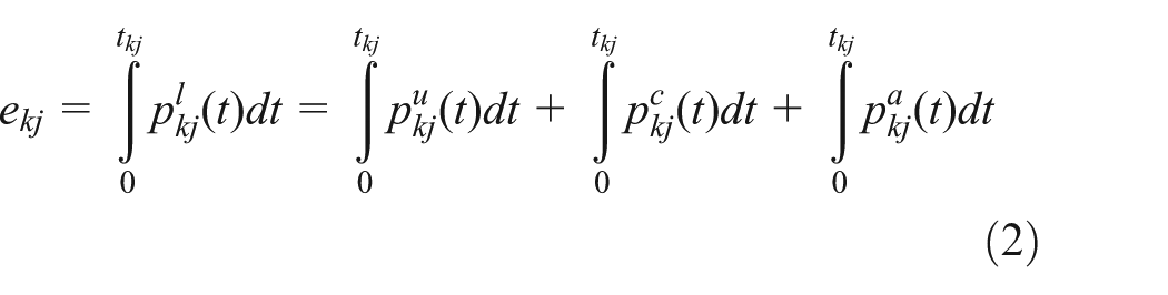
Assuming that the time of processing job j on machine k is tkj, then, according to equation (1), the energy consumption can be expressed as ekj
In practical applications, to facilitate the calculation and the actual operation, the idling power of a machine is often used in place of the output power of machining, and establishing an energy consumption matrix is feasible after practice.
The loading loss of power is caused by the loading condition of a machine, which is proportional to the output power pc in the allowable range. The power balance equation of machining can be expressed as

where α represents the loading power loss factor of the machine.
Therefore, equation (2) can be converted to the following equation

When the process parameters are the same, the energy consumption for machining the same parts is approximately the same, and the machining energy is not much greater than the idling energy consumption. Moreover, the impact of changing α is negligible compared to the energy consumed in the machining process. Therefore, the difference of the energy consumed in the machining process mainly loads from its idling consumption, so equation (4) can be simplified as follows

In variable machine parameters, the spindle revolution has a critical role in the idling power of machines; therefore, equation (5) could be further simplified as follows

In equation (6), pu(r) is relative to the spindle speed of machining. In other words, the total power can be replaced by the idle power pu(r) under different machine rotational speeds for the JSP.
Evaluation model of noise emission
Before evaluating the workshop noise, we must determine the evaluation index. Many physical indicators can be used to measure sound strength, such as sound pressure, sound pressure class, sound intensity, and sound intensity class. The most common indicator is sound pressure class, measured using the well-known unit of decibels (dB). For a machining shop, the noise radiation is wide band and stationary when all machines work at the same processing speed. A weighted method is used to correct such noise. Therefore, this article uses Class A sound pressure to evaluate the radiation of machining noise.
The noise of machining usually comprises structure noise and cutting noise; structure noise is typically evaluated by measuring the noise of idling machines, while cutting noise is due to the dynamic force of cutting. Cao and Yin reported that the cutting power consumption, dynamic cutting force, and cutting noise in the machining system could be regarded as approximately equal if using the same conditions of the process parameters, the fixture, and so on. The machining noise is mostly from the structure noise, which is determined by the machine frame. 27
Based on the reported studies, this article established a noise coefficient matrix of the scheduling model based on the spindle idling noise corresponding to the machine. 28 In the matrix lvw = lv(r), the machine idling noise parameter is associated with the spindle speed and irrelevant to parts.
After establishing the noise coefficient matrix in the scheduling model, we can obtain the noise figure of each machined workpiece. A schedule consists of a number of machining stages of the workpieces. This article uses an equivalent sound Class A to evaluate the noise performance merits in different scheduling environments.29,30
In equivalent sound Class A, actual noises rarely remain stable and fixed but rather fluctuate up and down over time. In general, acoustic energy within the averaging time of the cycle is used to obtain the average energy in each sound Class A of the fluctuated change happening in a certain period. Then a continuous and stable sound Class A in an equivalent period is selected to represent the loudness. This continuous and stable sound Class A is called an equivalent continuous sound class of the unstable noise, marked by leq, which approximates that leq works consistently in the period, and is also called equivalent continuous sound Class A or equivalent sound Class A. The definition of the equivalent continuous sound class is the formula
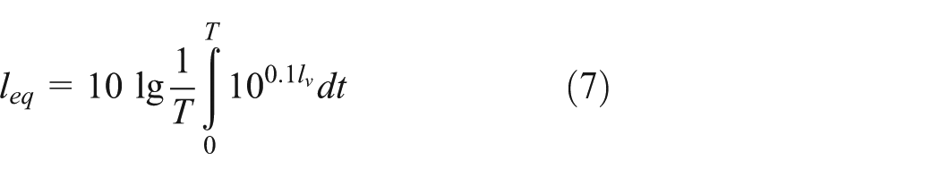
where lv is the instantaneous value of sound Class A in the exposure time and T is the exposure time of the noise.
In the workshop studied in this article, the radiated noise value in each period is stable when the machine processes at the spindle speed. Therefore, equation (7) can be rewritten as

where lv is the sound Class A measured in v paragraphed time and tv is the v paragraphed time.
Based on the above evaluation modes of productivity, energy consumption, and noise emission, a mixed integer programming model of the low-carbon JSP is proposed.
Mixed integer programming model of low-carbon JSP
The definition of the low-carbon JSP is as follows: a set of jobs J = {1, 2,…, n} are to be processed by a set of machines M = {1, 2,…, m}. The process of each job on each machine is pre-determined, and each job could be processed by a different machining speed according to the machine. The spindle speeds of a set of machines are represented by S = {s1, s2,…, ss}, corresponding to the machining time of each spindle speed. The idling power and noise are known. Two sub-problems exist in this model: one is to determine which machine will process the operation of each job, and the other one is to schedule all operations according to the three objectives.
To solve this problem, the following assumptions are made:
Jobs are independent. Job preemption is not allowed and each machine can handle only one job at a time.
The different operations of one job cannot be processed simultaneously.
All jobs and machines are simultaneously available at time 0.
After a job is processed on a machine, the job is immediately transported to the next machine on its process, and the transmission time is assumed to be negligible.
The setup time for the operations on the machines is independent of the operation sequence and is included in the processing times.
A turn off/on strategy is used to save energy when the machine is idle.
Based on these assumptions and the classical JSP model, the mixed integer programming model of the low-carbon JSP is proposed as follows:
The notations used to explain the model are described below:
n total number of jobs
m total number of machines
r spindle speed of machine,
i, j index of job, i, j = 1,2,…,n
h, k index of machine, h, k = 1,2,…,m
cik completion time of job i on machine k
pikr processing time of job i on machine k with spindle speed r
qikr total power that job i on machine k with spindle speed r (note that qikr is equal to the total power, while the total power is associated with idle power pu(r) according to equations (1)–(6). Therefore, qikr is equal to pu(r) in this article)
vikr machining noise of job i on machine k with spindle speed r
M sufficiently large positive number


Objectives:
Minimizing the makespan

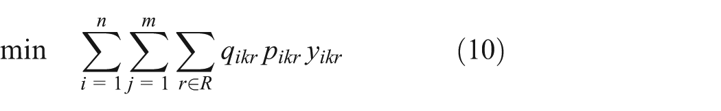
Minimizing the total energy consumption
Minimizing the noise emission

Subject to:
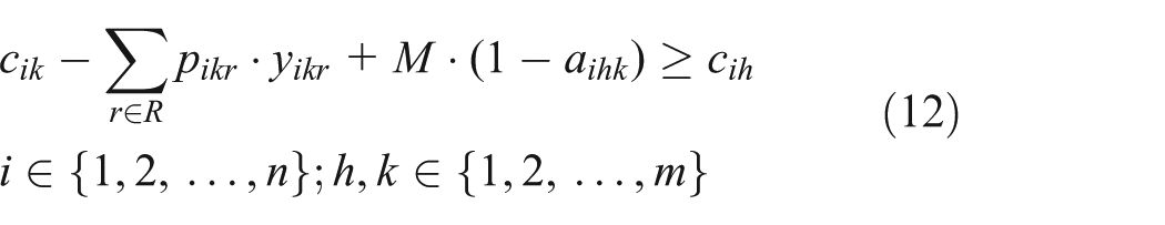
The different operations of one job cannot be processed simultaneously
Each machine can handle only one job at a time
The job cannot be preempted

Only one spindle speed for each operation should be selected

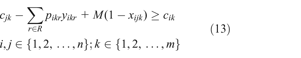
The objective functions are equations (9)–(11). Constraint (12) ensures that the different operations of one job cannot be processed simultaneously. Constraint (13) ensures that each machine can handle only one job at a time. Constraint (14) ensures that the job cannot be preempted. Constraint (15) ensures that only one spindle speed is selected for each operation.
The mixed integer programming model of the energy-efficient JSP developed above can be solved using the mixed integer programming methods. JSP has been proven to be one of the most difficult NP-complete problems. 31 The energy-efficient JSP is also an NP-complete problem. Finding perfect solutions for large problems in reasonable time is difficult. The model proposed in this article is a multi-objective optimization problem, so the problem considered in this article is very hard. To solve this problem effectively, this article proposes a MOGA based on a simplex lattice design to solve the model and obtains a set of solutions distributed evenly on the Pareto boundary.
MOGA based on a simplex lattice design for low-carbon JSP
Simplex lattice design
Simplex lattice design was used early in the design of mixing formulas. The goal of simplex lattice design is to reasonably distribute the weight of the individual components and to evenly distribute each mixing formula weight in the design space. Then the design is tested separately by each distribution weight to find the best production formulation. 32
If each side of an equilateral triangle in Figure 2(a) is bisected, as shown in Figure 2(b), the three vertices and three midpoints on each side of this triangle are called the second-order lattice point set, marked as {3, 2}, where “3” represents the number of vertices of the regular simplex, with fraction m = 3, and “2” represents the equivalent divided number on each side, so that the order d = 2.

Simplex lattice design.
If each side of the equilateral triangle is divided into three equal portions, as shown in Figure 2(c), the points are connected by a straight line that is parallel to one side, forming smaller equilateral triangle lattices within the original equilateral triangle. These vertices of the smaller equilateral triangles are called the third-order lattice point set, marked as {3, 3} in the simplex lattice design.
The other lattice point sets can be obtained by this approximate method. Selecting the above regular simplex as the design space of the test, if the points on the regular simplex lattice were chosen as the test points with response to the order, this test design would be called a simplex lattice point design. As known from the regular distribution of the simplex points in design space, this design can ensure that the test points distribute uniformly. In addition, the calculation becomes simpler and more precise.
The algorithm designed in this article applied the simplex lattice point design to various objective weight evaluations, obtained a set of evenly distributed weights using the design of simplex lattice points, guided the potential solution into various solution space directions, and finally obtained the uniform distribution Pareto set.
Simplex lattice design has 6 total points in the {3, 2} point set and 10 total points in the {3, 3} point set. As proven, there are
Encoding and decoding methods
Encoding and decoding methods significantly impact the algorithm performance. Effective encoding and decoding methods can make the algorithm operation easier and improve the calculation performance.
Each chromosome in a scheduling population consists of two parts with the same length, as shown in Figure 3. The first part of a chromosome is the scheduling string. In this article, the scheduling encoding consisting of the job numbers is the operation-based representation. This representation uses an unpartitioned permutation with Si repetitions of job numbers (where Si is the total number of operations for job i). In this representation, each job number appears Si times in the chromosome. By scanning the chromosome from left to right, the fth appearance of a job number refers to the fth operation of this job. The important feature of this representation is that any permutation of the chromosome can be decoded to a feasible solution. This article assumes that there are n jobs. Then the length of the scheduling plan string is equal to

The chromosome of the problem.
The second part of a chromosome is the speed string. The length of this string is equal to the length of the scheduling string and denotes the selected spindle set of the corresponding operations of all jobs in the scheduling string.
Figure 3 shows an example chromosome. In this example, n is equal to 3, and S1 = S2 = S3 = 3. Therefore, the scheduling string and speed string are made up of nine elements each. For job 1, there are three operations, so three elements of the scheduling string are one. The other elements in the chromosome can be deciphered accordingly.
The permutations can be decoded into semi-active, active, non-delay, and hybrid schedules. The active schedule is adopted in this article. The decoding procedure is as follows: first, scan the scheduling string from left to right, reading the speed information of each operation corresponding to the gene located in the speed string (the speed information can obtain the processing time, energy consumption and noise emission); then insert all the operations sequence and order of the scanned chromosome into the earliest idle time corresponding to the machine that will process this operation. This procedure is followed until all the operations are arranged in the best available station. Meanwhile, the energy consumption of all the process sequences is summed, and noises are equivalently converted to sound Class A.
Initial population and fitness evaluation
The encoding principle of the scheduling string in the chromosome in this article is an operation-based representation. The important feature of this representation is that any permutation of the chromosome can be decoded to a feasible schedule. Permutations cannot break the constraints on the precedence relations of operations. The initial population is randomly generated based on the encoding principle.
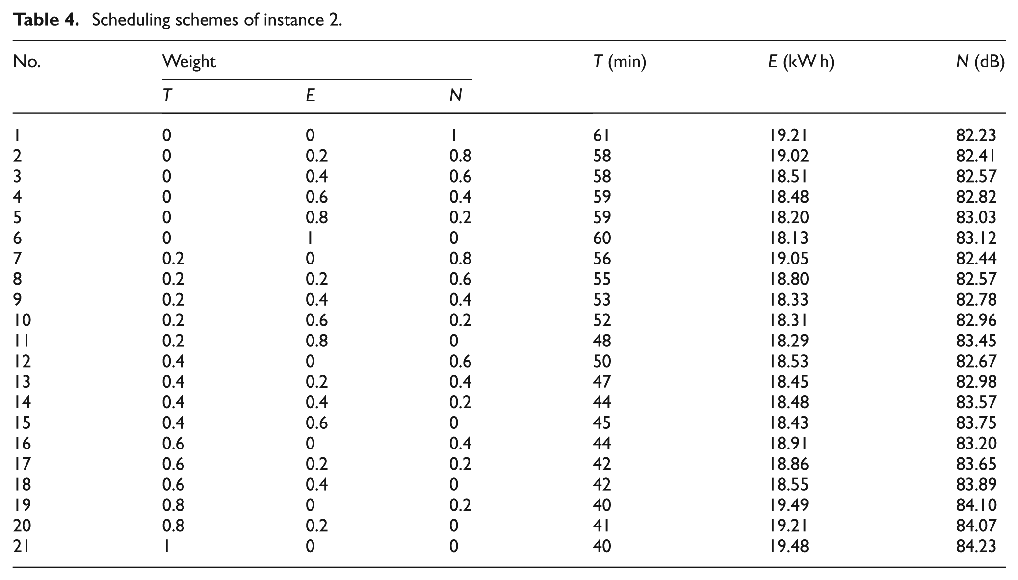
Because this is a multi-objective optimization problem, the fitness function should be combined with the makespan, energy consumption, and noise emission. For a scheduling plan, the maximum makespan is T(x), the total energy consumption is E(x), the equivalent sound Class A is N(x), and the fitness function could then be expressed as follows

where w1, w2, and w3 are the weight coefficients of each target and w1 + w2 + w3 = 1.
However, because the dimension of each objective function is not consistent, it cannot be summed directly. Moreover, the differences among the objective values are large, which easily allows the fitness function to be dominated by a single objective. Therefore, each objective should be distributed with dimensionless and normalized uniformity. After the fitness function is made dimensionless and normalized, equation (16) is rewritten as follows

where Tmax and Tmin denote the maximum and the minimum of objective T that can be achieved, respectively. The other parameters denote its significance similarly. After the disposal of equation (17), the range of each objective will be between 0 and 1. The fitness function also stays between 0 and 1, and the value of the fitness function approaches 0 for the same weight of a group, indicating that the scheduling plan performance improves.
To obtain a plurality of scheduling plans, the weight coefficients of the fitness function w1, w2, and w3 are not unique. Their values are generated by the simplex lattice point design described in section “Simplex lattice design.”
Genetic operations
Selection operation
The proportional selection method is used as the selection operation. Using the probability of the proportion to individual fitness levels to select appropriate individuals, the method generates the random,
Crossover operation
The single-point crossover method is used for the crossover operations, with the following steps (an example is shown in Figure 4):
Step 1: randomly select two individuals in the population as parents A and B and generate a random integer x following the length l of the front portion of chromosome string, where 1 < x < l.
Step 2: exchange the gene locus of the front portion and the rear portion of parents A and B before gene X and generate the children A and B, respectively.
Step 3: scan the excess and the missing genes in the front portion of the children chromosomes A and B, use the missing genes to modify the excess genes, and adjust the modified genes according to the revolution of the front individual of the crossover to ensure the legitimacy of the chromosome.
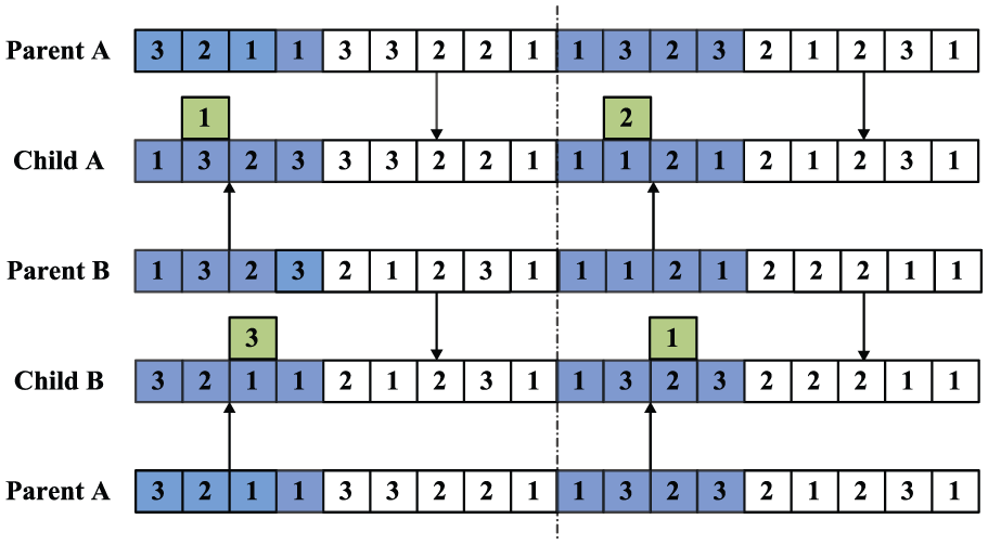
Crossover operation.
Mutation operation
The mutation operation is divided into two parts. The detailed steps are as follows (an example is shown in Figure 5):
Step 1: for the first part of the parent chromosomes, randomly select two positions and mutually exchange the sequences in the two positions. Meanwhile, exchange the genes in the rear part of the chromosomes that represent the revolution information mutually as well.
Step 2: for the rear parts of the parent chromosome, randomly select a gene representing the revolution information if it has various revolution selections and randomly select the rest.

Mutation operation.
A basic schematic of the mutation process is described as follows.
Elite strategy
To maintain the number of outstanding individuals in the population or species and ensure that the algorithm quickly converges to the optimal solution, the quality protection strategy is normally used in the algorithm. The best individual of the fitness is selected from the parent generation G of proportions during the evolution of each generation of the population and, directly entering the next generation of the population, the individuals of the remaining proportion (I-G) are generated by the mutation operation of crossover. This process ensures that the individuals of the offspring population and the parent population are consistent.
Framework of the proposed MOGA for the low-carbon JSP
Based on the key operations described above, the working steps of the algorithm procedure are as follows (the flowchart is shown in Figure 6):
Step 1: randomly generate an initial population and set parameters, including the simplex lattice design order d, the number of individuals of population NIND, the maximum iteration number MAXGEN, the quality protection ratio G, the crossover probability XOVR, and the mutation probability MUTR.
Step 2: calculate the fitness value of each individual in the population to determine whether the algorithm termination condition is satisfied or not. If the condition is satisfied, output the optimal results. Otherwise, perform the following steps.
Step 3: compare the pros and cons of the fitness value for each individual in the population and perform the operation of quality protection to select a better individual for the proportion G of fitness. Directly enter the next generation of the population.
Step 4: perform the selection operation on the population; select two parent individuals by a certain probability according to the fitness value of the individuals.
Step 5: perform the crossover operation on the selected parent individuals using the crossover probability XOVR to generate two interim individuals.
Step 6: MUTR performs the mutation operation on the interim individuals using the mutation probability. Generate two children individuals and put them into the next-generation population.
Step 7: check the number of individuals in the new generation population m. If m < NIND, return to Step 4; if m = NIND, replace the old population with the new generation population, add one to the generation number, and return to Step 2.

The flowchart of the MOGA.
Experimental studies and discussion
The proposed algorithm was coded in MATLAB programming and implemented on a computer with a 2.0 GHz Core (TM) 2 Duo CPU. The algorithm designed in section “MOGA based on a simplex lattice design for low-carbon JSP” applied the simplex lattice point design to various objective weight evaluations, obtained a set of evenly distributed weights using the design of simplex lattice points, guided the potential solution into various solution space directions, and finally obtained the uniform distribution Pareto set. To evaluate the performance of this method, three instances with different scales are designed.
Experiment 1 (4 × 5)
Table 1 illustrates the data of instance 1.
Data of instance 1 (4 jobs and 5 machines).

In the solution, first take the maximum makespan, total processing energy consumption, and equivalent sound Class A of an individual objective and optimize them to obtain Tmin = 22, Tmax = 35; Emin = 4.82, Emax = 6.79; and Nmin = 77.80, Nmax = 84.80. Thus, the fitness function of the algorithm changes to the following

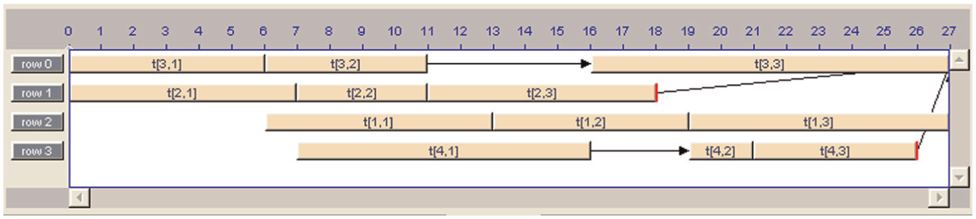
During the algorithm operation, set the relevant parameters to the following: the simplex lattice point design order d = 5, the number of population individuals NIND = 100, the evolution algebra order MAXGEN = 200, the quality protection ration G = 10%, the crossover probability XOVR = 0.8, and the mutation probability MUTR = 0.6. After operating the algorithm through many iterations, obtain the problem solution set, as shown in Table 2. Figure 7 shows the space distribution of the solution set, and Figure 8 shows the Gantt chart of scheduling scheme 13.
Scheduling schemes of case 1.

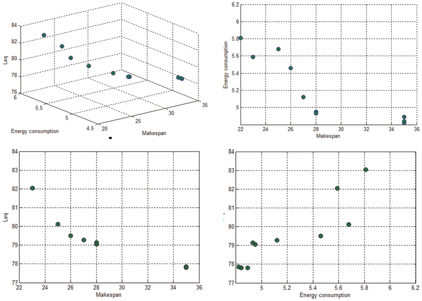
Scatter plot of scheduling schemes of instance 1.

The Gantt chart of the 13th scheduling scheme of instance 1.
The proposed MOGA is compared with the exact algorithm provided by IBM ILOG CPLEX CP Optimizer tool 12.5 (CP optimizer) for this instance, and the results obtained by the exact method are presented in Figure 9. When only the makespan criteria are considered, the makespan obtained by the MOGA is 22 min, while that obtained by the exact algorithm is 27. Therefore, the proposed MOGA is superior to the exact algorithm.
The Gantt chart obtained by the exact algorithm.
Experiment 2 (10 × 6)
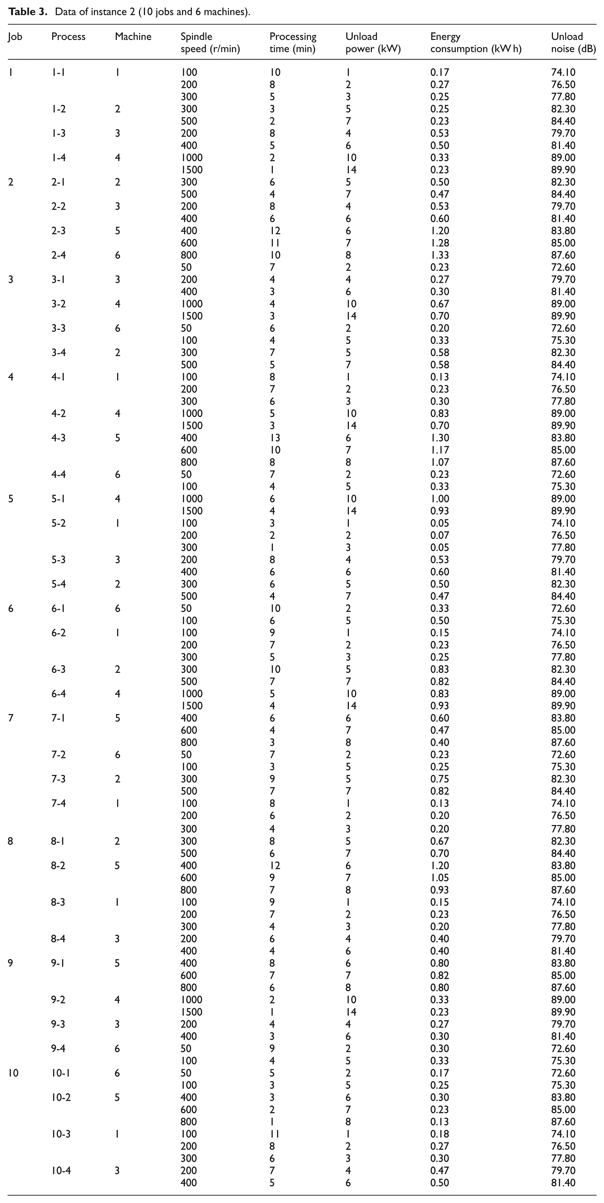
Table 3 illustrates the data of instance 2.
Data of instance 2 (10 jobs and 6 machines).
In the solution, first take the maximum makespan, total processing energy consumption, and equivalent sound Class A for an individual target and optimize them to obtain Tmin = 40, Tmax = 61; Emin = 18.13, Emax = 20.81; and Nmin = 82.23, Nmax = 84.58. Thus, the fitness function of the algorithm is as follows
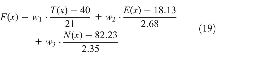
During the algorithm operation, set the relevant parameters to the following: the simplex lattice point design order d = 5, the number of population individuals NIND = 300, the evolution algebra order MAXGEN = 200, the quality protection ration G = 10%, the crossover probability XOVR = 0.9, and the mutation probability MUTR = 0.8. After operating the algorithm through many iterations, the problem solution set is shown in Table 4. Figure 10 shows the space distribution of the solution set, and Figure 11 shows the Gantt chart of scheduling scheme 15.
Scheduling schemes of instance 2.

Scatter plot of scheduling schemes of instance 2.

The Gantt chart of the 15th scheduling scheme of instance 2.
Experiment 3 (20 × 5)
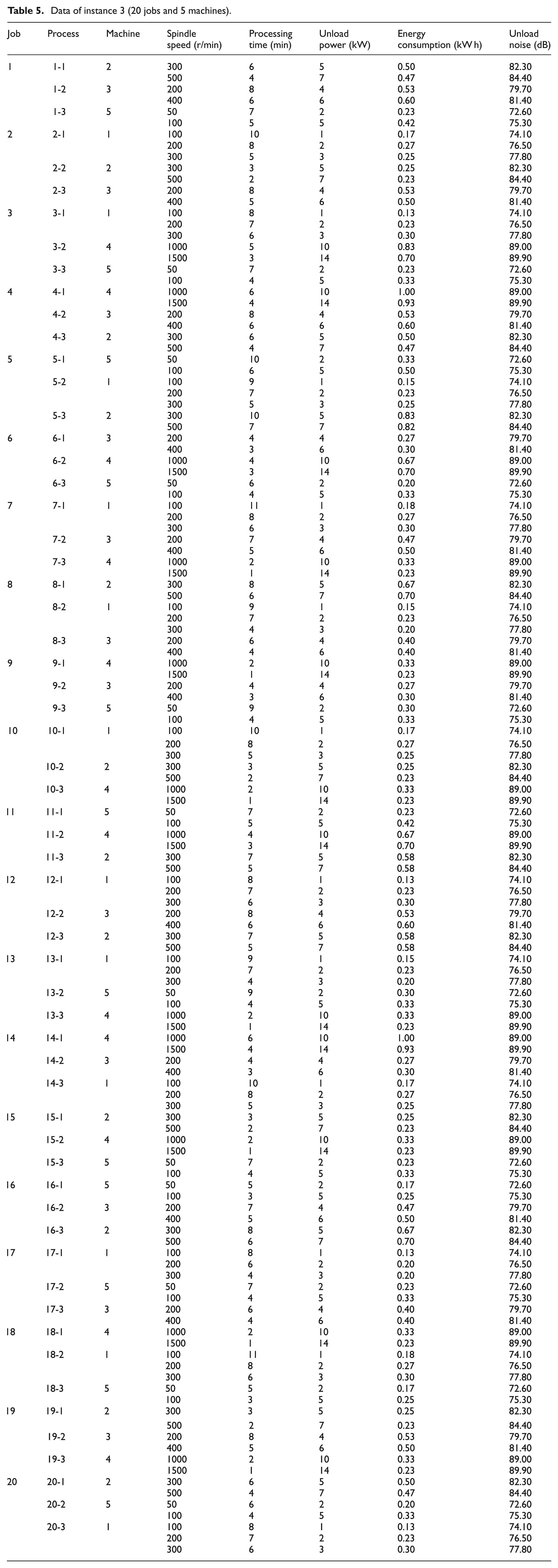
Table 5 illustrates the data of instance 3.
Data of instance 3 (20 jobs and 5 machines).
In the solution, first take the maximum makespan, total processing energy consumption, and equivalent sound Class A for an individual target and optimize them to obtain Tmin = 64, Tmax = 110; Emin = 21.73, Emax = 24.81; and Nmin = 81.57, Nmax = 83.14. Thus, the fitness function of the algorithm is as follows

During the algorithm operation, set the relevant parameters to the following: the simplex lattice point design order d = 5, the number of population individuals NIND = 500, the evolution algebra order MAXGEN = 200, the quality protection ration G = 10%, the crossover probability XOVR = 0.9, and the mutation probability MUTR = 0.8. After operating the algorithm through many iterations, the problem solution set is shown in Table 6. Figure 12 shows the space distribution of the solution set, and Figure 13 shows the Gantt chart of scheduling scheme 15.
Scheduling schemes of instance 3.


Scatter plot of scheduling schemes of instance 3.

The Gantt chart of the 15th scheduling scheme of instance 3.
Performance comparison
In this section, three indexes are used to test the effectiveness of the MOGA. Three indexes are used in this article, which are described as follows:
1. Generational distance (GD) indicates how far away the Pareto front (PF) found is from the PF*. 33 This metric is formulated as follows
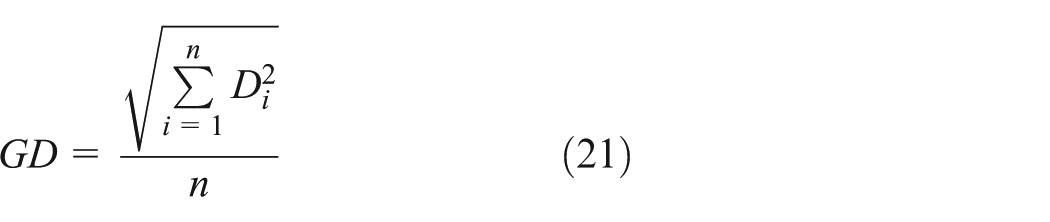
where n is the number of PF points found so far, and
2. Inverse generation convergence (IGD) is the inverse convergence method of the GD method. IGD calculates the mean of the minimum distance between the Pareto surface with points spread uniformly and the non-dominated solution sets. 34 The formulation of IGD is as follows
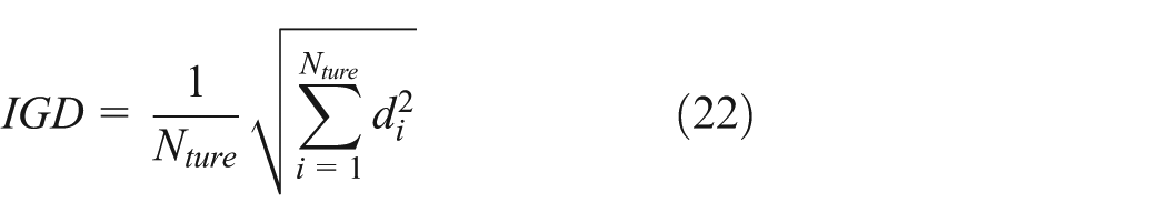
where
3. Spread (Δ) is applied to evaluate the distribution of the PF solution set and can be defined as follows 33
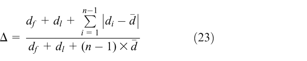
where
To test the efficiency of the proposed algorithm, it is compared with a well-known multi-objective evolutionary algorithm (MOEA) such as non-dominated sorting genetic algorithm II (NSGA-II) for the aforementioned cases. Tables 7–9 show the mean and standard deviation metrics for these algorithms more than 30 independent runs. Tables 7–9 reveal that the MOGA outperforms NSGA-II with regard to all metrics. Therefore, the MOGA is very suitable for solving this type of scheduling problem.
GD indicator.

MOGA: multi-objective genetic algorithm; NSGA-II: non-dominated sorting genetic algorithm II.
IGD indicator.

MOGA: multi-objective genetic algorithm; NSGA-II: non-dominated sorting genetic algorithm II.
Spread indicator.
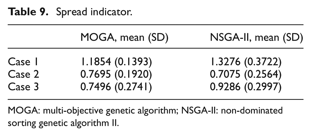
MOGA: multi-objective genetic algorithm; NSGA-II: non-dominated sorting genetic algorithm II.
Parameters and operator analysis
In the MOGA, the algorithm performance is sensitive to the value of the parameters such as the crossover and mutation probability. However, the two parameters are not constant. In general, the crossover rate is set to the larger value, within a range of 0.7–0.9, while the mutation rate is usually set to the smaller value between 0.4 and 0.8. To test how the parameter settings affect the algorithm performance, we set different parameter values of crossover and mutation probability while the other parameter settings are kept constant, where crossover probability XOVR = {0.7, 0.8, 0.9} and mutation probability MUTR = {0.4, 0.6, 0.8}. Figure 14 shows the changes in the objective (i.e. F(x)) with different crossover and mutation probabilities for case 2. The figure clearly shows that the gap between the best and the worst value is not significant. Therefore, although different parameter settings affect the behavior of the algorithm in this case, the effect is not significant. In addition, XOVR (single-point crossover rate) or MUTR (the proposed swap mutation rate) with larger values will positively affect the algorithm performance.
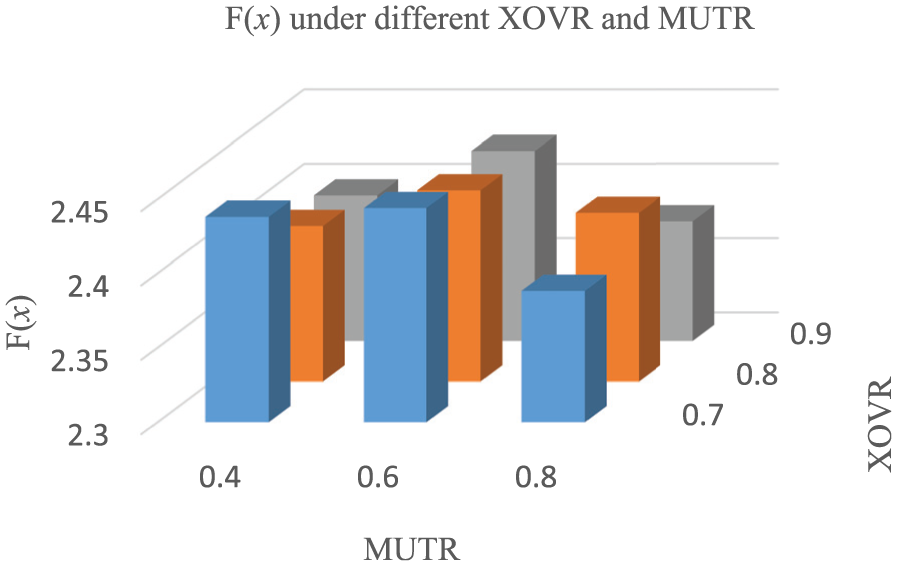
Parameter analysis for case 2.
Analysis of variance (ANOVA) can be used to calibrate the parameters. To test the efficiency of the proposed algorithm, it is used to find out the factors which have a significant impact on the algorithm through the data analysis. When the p-value of ANOVA is less than 0.05, the effect is significant. Table 10 show the F(x) and p metrics for the algorithm more than 30 independent runs. The results showed that MUTR and XOVR had no significant effect on the objective function. This is consistent with the above analysis.
MOGA parameters analysis of variances for case 2.

In addition, crossover has an important role in solving the scheduling problem. Different crossover operators are generally accepted to show different performance. To test the performance of the proposed algorithm, an algorithm with different crossover operators is measured. In this experiment, the MOGA is compared with an algorithm with partial mapping crossover (PMX). Each experiment conducted 10 independent runs for each case, and a boxplot is used to analyze the problem objective (i.e. F(x)).
Figure 15 shows that the MOGA with single-point crossover is more stable than that with PMX. Figure 16 shows that the average result obtained by the MOGA with one-point crossover is smaller than that of the result with PMX. Therefore, with increasing problem scale, one-point crossover is not sensitive to problem scale, but problem scale affects PMX.

Boxplot for different crossovers on MOGA for case 1.

Boxplot for different crossovers on MOGA for case 2.
Result analysis and discussion
An energy-efficient JSP issue comprises n jobs (each job contains ni operations, where ni is the total number of operations of job i) and m machines (each machine contains r spindle speeds for selection). The scale of the solution space is
In this article, a MOGA based on the simplex lattice point design is used to solve the proposed energy-efficient JSP model. The aim of the algorithm is to find a group uniform distribution scheduling scheme set. The results of the above three instances with different scales demonstrate the effectiveness of the proposed model and method for the low-carbon JSP. The energy-efficient scheduling method described in this article could provide more selective scheduling schemes for decision-makers. In addition, the scheduling scheme can be reasonably adjusted according to actual production requirements and changes in production targets to better guide production.
Conclusion and future studies
For the urgent demand of sustainable development in the modern manufacturing industry, this article proposed a new energy-efficient scheduling mathematical model considering productivity, energy efficiency, and noise reduction with variable spindle speed for the job shop environment. This model considers the machining spindle speed that impacts the production time, power, and noise to be flexible and an independent decision-making variable. This model presents the evaluation methods of productivity, energy consumption, and noise. To effectively solve this mixed integer programming model, an effective MOGA based on simplex lattice design is proposed. The corresponding encoding/decoding method, fitness function, and crossover/mutation operators are designed according to the features of this problem. To evaluate the performance of this method, three instances with different scales have been designed. The results demonstrate the effectiveness of the proposed model and method for the low-carbon JSP.
Based on the above study, the authors believe that further study of energy-efficient scheduling problems can be performed in the following three directions: (1) energy-efficient scheduling involves many indicators. Other low-carbon indicators could be considered in future studies, such as peak power and exhaust emissions. (2) For various manufacturing plants, more types of manufacturing plants (such as open workshops) can be considered in the future. (3) Adding dynamic factors to energy-efficient scheduling will bring the model closer to reality because the actual plant accompanies factors during processing such as job delay, precedence of urgent jobs, and machine breakdowns.
Footnotes
Academic Editor: Murat Uzam
Declaration of conflicting interests
The author(s) declared no potential conflicts of interest with respect to the research, authorship, and/or publication of this article.
Funding
The author(s) disclosed receipt of the following financial support for the research, authorship, and/or publication of this article: This work was supported by the National Natural Science Foundation of China (NSFC) under grant no. 51375004, National Key Technology Support Program under grant no. 2015BAF01B04, Youth Science & Technology Chenguang Program of Wuhan under grant no. 2015070404010187, and the Fundamental Research Funds for the Central Universities, HUST: grant no. 2015TS061, the Humanities and Social Sciences Foundation of Ministry of Education of China (grant no. 15YJC630162).