Chebyshev wavelet method to nonlinear fractional Volterra–Fredholm integro-differential equations with mixed boundary conditions

Abstract

This research work addresses the numerical solutions of nonlinear fractional integro-differential equations with mixed boundary conditions, using Chebyshev wavelet method. The basic idea of this work started from the Caputo definition of fractional differential operator. The fractional derivatives are replaced by Caputo operator, and the solution is approximated by wavelet family of functions. The numerical scheme by Chebyshev wavelet method is constructed through a very simple and straightforward way. The numerical results of the current method are compared with the exact solutions of the problems, which show that the proposed method has a strong agreement with the exact solutions of the problems. The numerical solutions of the present method are also compared with steepest decent method and Adomian decomposition method. The comparison with other methods reveals that this method has the highest degree of accuracy than those methods.

Introduction

Many important problems in fluid mechanics, viscoelasticity, electromagnetic, and other fields of science and engineering are modeled by fractional differential and integral equations.^1,2 Due to the real facts of its applications in different areas of research, the researchers have taken keen interest in the study of fractional calculus. In this context, the Volterra–Fredholm fractional integro-differential equations have an important role in various fields of biomechanics, elasticity, economics, fluid dynamics, heat and mass transfer, oscillation theory, and airfoil theory.^3,4 The challenging work is to find the solution while dealing with Volterra–Fredholm fractional integro-differential equations. Therefore, many researchers have tried their best to use different techniques to find the analytical and numerical solutions of these problems, for example, Adomian decomposition method (ADM), ⁵ spline collocation method (SCM), ⁶ fractional transform method (FTM), ⁷ homotopy perturbation method (HPM), ⁸ operational tau method (OTM), ⁹ shifted Chebyshev polynomial method (SCPM), ¹⁰ rationalized Haar function method (RHFM), ¹¹ exp-function method, ¹² traveling wave transformation method, ¹³ and Cole–Hopf transformation method, ¹⁴ and also see the work in Yang et al., ¹⁵ Sayevand and Pichaghchi, ¹⁶ and Wang and Liu. ¹⁷ Recently, Yang et al. ¹⁸ did a comprehensive study of the methods which have been used for the solutions of the problems containing fractional derivatives and integral operators.

Besides these methods, most of the authors have applied a comparatively new numerical techniques based on wavelets.^19–22 The methods based on Chebyshev wavelets have gained much importance during the last decade because of its simple, effective, and straightforward implementation. Therefore, the researcher paid great attention to these methods to solve problems in different fields of science and engineering, for example, Chebyshev wavelet operational matrix (CWOM), ²³ Chebyshev finite difference method (CFDM), ³ SCPM, ¹⁰ and Chebyshev wavelet method (CWM).^24,25

In this article, an efficient CWM is used to obtain the numerical solutions of some Volterra–Fredholm fractional integro-differential equations. The simulations are performed by the proposed method easily. The numerical results found by the present method are compared with other numerical methods, showing the greatest degree accuracy than any other method.

Preliminaries and definitions

To continue with this work, we present some definitions and other mathematical preliminaries. These concepts play very massive role to complete this work.

Definition 1

The Riemann fractional integral operator $I^{\mu }$ of order $\gamma$ on the usual Lebesgue space $L_1[a,b]$ is given by

$$\left(I^{\mu }g\right)\left(t\right)=\frac{1}{\mathrm{\Gamma }\left(\mu \right)}\underset{0}{\overset{t}{\int }}{(t-\xi )}^{\mu -1}g\left(\xi \right)d\xi ,\gamma >0$$

(1)

where $(I^{0}g)(t)=g(t)$ .

This integral operator has the following properties

$$\begin{array}{c}{I}^{\mu }{I}^{\eta }=I^{\mu +\eta }\hfill \\ I^{\mu }{I}^{\eta }=I^{\eta }{I}^{\mu }\hfill \\ I^{\mu }{(t-a)}^{\upsilon }=\frac{\mathrm{\Gamma }(\upsilon +1)}{\mathrm{\Gamma }(\mu +\upsilon +1)}{(t-a)}^{\mu +\upsilon }\hfill \end{array}$$

where $L_1[a,b]$ , $\alpha$ , $\mu \ge 0$ , and $\upsilon >-1$ .

Definition 2

The Riemann fractional derivative of order $\mu >0$ is defined as

$$\left(D^{\mu }g\right)\left(t\right)={\left(\frac{d}{\mathrm{dt}}\right)}^n\left(I^{n-\mu }g\right)\left(t\right),n-1<\mu \le n$$

where n is an integer.

However, the Riemann fractional derivative has certain drawbacks due to which Caputo proposed a modified differential operator.

Definition 3

The Caputo definition of fractional differential operator is given by

$$\left(D^{\mu }g\right)\left(t\right)=\frac{1}{\mathrm{\Gamma }(n-\mu )}\underset{0}{\overset{t}{\int }}{(t-\xi )}^{n-\mu -1}{g}^{\left(n\right)}\left(\xi \right)d\xi ,n-1〈\mu 〉n$$

where $t>0,n$ is an integer.

It has the following two basic properties

$$\begin{array}{c}\left(D^{\mu }{I}^{\mu }g\right)\left(t\right)=g\left(t\right)\hfill \\ \left(I^{\mu }{D}^{\mu }g\right)\left(t\right)=\left(g\right)\left(t\right)-{(x+a)}^n\hfill \\ =\sum _{k=0}^n{f}^{\left(k\right)}\left(0^{+}\right)\frac{{(t-a)}^k}{k!},t>0\hfill \end{array}$$

Properties of the Chebyshev wavelets

Wavelets consist of family of functions generated from the dilation m and translation l of a single function $\psi (x)$ called the mother wavelet. When the dilation a and translation b change continuously, then we obtain the following continuous family of wavelet ²⁶

$${\psi }_{l,m}\left(x\right)={\left|a\right|}^{\frac{1}{2}}\psi \left(\frac{x-l}{m}\right),l,m\in R,m\ne 0$$

If we restrict the parameters l and m to discrete values as

$$m=a_0^{-k},l=n{b}_0{a}_0^{-k},a_0>1,b_0>1$$

We have the following family of discrete wavelets

$${\psi }_{k,n}\left(x\right)={\left|a\right|}^{\frac{k}{2}}\psi (a_0^{k}x-n{b}_0),k,n\in Z$$

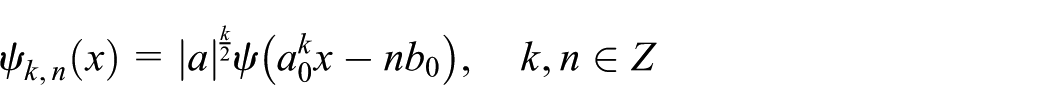
where ${\psi }_{k,n}$ forms a wavelet basis for $L^2(R)$ . Especially, when $a_0=2$ and $b_0=1$ , then ${\psi }_{k,n}(x)$ forms an orthogonal basis.

The second kind of Chebyshev wavelets is constituted of four parameters, ${\psi }_{n,m}(x)=\psi (k,n,m,x)$ , where $n=1,2,\dots ,2^{k-1}$ , k is any positive integer, and m is the degree of the second Chebyshev polynomial. The Chebyshev wavelets are defined on the interval $0\le x<1$ as

$${\psi }_{n,m}\left(x\right)=\{\begin{array}{cc}{2}^{\raisebox{1ex}{$k$}\!\left/ \!\raisebox{-1ex}{$2$}\right.}\tilde{T}\left(2^k-2n+1\right),& \frac{n-1}{2}\le x\le \frac{n+1}{2}\\ 0,& otherwise\end{array}$$

where

$$\widetilde{T_m}\left(x\right)=\sqrt{\frac{2}{\pi }}{T}_m\left(x\right),m=0,1,2,\dots ,M-1$$

(2)

Here, $T_m(x)$ are the second Chebyshev polynomials of degree m with respect to the weight function in the interval [−1, 1] and satisfying the following recursive formula

$$\begin{array}{c}{T}_0\left(x\right)=1,T_1\left(x\right)=2x\hfill \\ T_{m+1}\left(x\right)=2x{T}_m\left(x\right)-T_{m-1}\left(x\right),m=1,2,3,\dots \hfill \end{array}$$

CWM

In this article, we consider the fractional integro-differential equations of the form

$$\begin{array}{l}{\displaystyle \sum _{i=0}^m{\mu }_i}\left(x\right)y^{\left(i\right)}\left(x\right)=f\left(x\right)+{\lambda }_1{\displaystyle \underset{0}{\overset{x}{\int }}{k}_1}\left(x,t\right){\left(y\left(t\right)\right)}^{p}dt\\ +{\lambda }_2{\displaystyle \underset{a}{\overset{b}{\int }}{k}_2}\left(x,t\right){\left(y\left(t\right)\right)}^{q}dt=0\end{array}$$

(3)

With the initial conditions given by

$$y^{\left(i\right)}\left(a\right)=y_i$$

For $i=1,2,3,\dots ,m-1$ , ${\lambda }_1$ , ${\lambda }_2$ , and $y_i$ are constants and p, $q\in \mathrm{Z}$ . $f(x)$ , $k_1(x,t)$ , $k_2(x,t)$ , $y(x)$ , and ${\mu }_i(x)$ are known functions of x. These functions are differentiable in $a\le x\le t\le b$ .

The solution to equation (3) can be extended by Chebyshev wavelets series as

$$y\left(x\right)=\sum _{n=1}^{\infty }\sum _{m=0}^{\infty }{c}_{n,m}{\psi }_{n,m}\left(x\right)$$

(4)

where ${\psi }_{n,m}(x)$ is given by equation (1). The series in equation (4) is truncated to finite number of terms that is

$$y_{k,M}\left(x\right)=\sum _{n=1}^{2^{k-1}}\sum _{m=0}^{M-1}{c}_{n,m}{\psi }_{n,m}\left(x\right)$$

(5)

This shows that there are $2^{k-1}M$ conditions to determine $2^{k-1}M$ coefficients, $c_{i,j}$ .

In this article, we have considered some initial and mixed boundary value fractional integro-differential equations of order less than one. There are two conditions for mixed boundary value problem. The mixed boundary conditions are approximated by CWM as given in the following equations.

The first mixed boundary condition is approximated as

$$\begin{array}{l}{\displaystyle \sum _{n=1}^{2^{k-1}}{\displaystyle \sum _{m=0}^{M-1}{c}_{n,m}}}{\psi }_{n,m}\left(0\right)+{\displaystyle \sum _{n=1}^{2^{k-1}}{\displaystyle \sum _{m=0}^{M-1}{c}_{n,m}}}{\psi }_{n,m}\left(1\right)\\ +{\displaystyle \sum _{n=1}^{2^{k-1}}{\displaystyle \sum _{m=0}^{M-1}{c}_{n,m}}}\psi {\prime }_{m,n}\left(0\right)+{\displaystyle \sum _{n=1}^{2^{k-1}}{\displaystyle \sum _{m=0}^{M-1}{c}_{n,m}}}\psi {\prime }_{m,n}\left(1\right)={\alpha }_0\end{array}$$

(6)

and the second is

$$\begin{array}{l}{\displaystyle \sum _{n=1}^{2^{k-1}}{\displaystyle \sum _{m=0}^{M-1}{c}_{n,m}}}{\psi }_{n,m}\left(0\right)+{\displaystyle \sum _{n=1}^{2^{k-1}}{\displaystyle \sum _{m=0}^{M-1}{c}_{n,m}}}{\psi }_{n,m}\left(1\right)\\ +{\displaystyle \sum _{n=1}^{2^{k-1}}{\displaystyle \sum _{m=0}^{M-1}{c}_{n,m}}}\psi {\prime }_{m,n}\left(0\right)+{\displaystyle \sum _{n=1}^{2^{k-1}}{\displaystyle \sum _{m=0}^{M-1}{c}_{n,m}}}\psi {\prime }_{m,n}\left(1\right)={\beta }_0\end{array}$$

(7)

The remaining $2^{k-1}M-2$ conditions can be obtained by substituting equation (5) into equation (3), and we obtain

$$\begin{array}{l}\frac{d^a}{d{x}^a}{\displaystyle \sum _{i=0}^m{\mu }_i\left(x\right)}{\displaystyle \sum _{n=1}^{2^{k-1}}{\displaystyle \sum _{m=0}^{M-5}{c}_{n,m}{\psi }_{n,m}\left(x_i\right)}=f\left(x\right)}\\ +{{\displaystyle \underset{0}{\overset{x}{\int }}\left({\displaystyle \sum _{n=1}^{2^{k-1}}{\displaystyle \sum _{m=0}^{M-5}{c}_{n,m}{\psi }_{n,m}}\left(x_i\right)}\right)}}^{p}dt+{\lambda }_2{\displaystyle \underset{a}{\overset{b}{\int }}{k}_2}\left(x,t\right)\\ {\left({\displaystyle \sum _{n=1}^{2^{k-1}}{\displaystyle \sum _{m=0}^{M-11}{c}_{n,m}}}{\psi }_{n,m}\left(x_i\right)\right)}^{q}dt=0\end{array}$$

(8)

Assume that equation (6) is exact at $2^{k-1}M-2$ at $x_i$ points, the $x_i$ points are calculated by the following formula

$$x_i=\frac{i-0.5}{2^{k-1}M}\mathrm{for}i=1,2,3,\dots ,2^{k-1}M-2$$

The combination of equations (6)–(8) forms the linear system of $2^{k-1}M$ linear equations. The unknown $c_{i,j}$ are calculated through the solution of this system of equations. The same procedure can be repeated for other initial value of Volterra–Fredholm fractional integro-differential equations.

Numerical examples

Example 1

Consider the following fractional order nonlinear boundary value problem ²⁷

$$\begin{array}{l}\frac{d^{\sqrt{3}}y}{d{x}^{\sqrt{3}}}-\frac{2}{\mathrm{\Gamma }\left(3-\sqrt{3}\right)}{x}^{\left(2-\sqrt{3}\right)}-2\sin x\\ +2x-{\displaystyle \underset{0}{\overset{x}{\int }}\cos }\left(x-t\right)y\left(t\right)dt=0,0\le x\le 1\end{array}$$

With mixed boundary conditions

$$y\left(0\right)+y\left(1\right)-y\prime \left(0\right)-y\prime \left(1\right)=-1$$

and

$$3\mathrm{y}\left(0\right)+4\mathrm{y}\left(1\right)+\mathrm{y}\prime \left(0\right)-3\mathrm{y}\prime \left(1\right)=-2$$

The exact solution is

$$y\left(x\right)=x^2$$

In Table 1, the exact solution and approximate solution by CWM of example 1 are represented by y (exact) and y (CWM), respectively (Figure 1). The CWM is applied for $M=19$ and $K=1$ . The approximate solutions are compared with the exact solution of problem. The errors associated with steepest decent method and CWMs are denoted by error (SDM) and error (CWM), respectively. The error analysis from this table shows that CWM has higher accuracy than ADM (Figure 2).

Table 1.

The numerical results of Example 1.

$x_i$	y (exact)	y (CWM)	Error (ADM) 20	Error (CWM)
0.0	0.00000000000000000000	0.00000000000000000427		4.26E−18
0.1	0.01000000000000000000	0.01000000000000000119		1.19E−18
0.2	0.04000000000000000000	0.03999999999999999841	7.31E−9	1.58E−18
0.3	0.09000000000000000000	0.08999999999999999614		3.85E−18
0.4	0.16000000000000000000	0.15999999999999999413	7.00E−9	5.87E−18
0.5	0.25000000000000000000	0.24999999999999999226		7.74E−18
0.6	0.36000000000000000000	0.35999999999999999049	6.74E−9	9.51E−18
0.7	0.49000000000000000000	0.48999999999999998878		1.12E−17
0.8	0.64000000000000000000	0.63999999999999998711	6.55E−9	1.28E−17
0.9	0.81000000000000000000	0.80999999999999998544		1.45E−17
1.0	1.00000000000000000000	0.99999999999999998375	6.49E−9	1.62E−17

CWM: Chebyshev wavelet method; ADM: Adomian decomposition method.

Figure 1.

The graph of exact solution versus Chebyshev wavelet approximation of Example 1.

Figure 2.

The graph of errors obtained by ADM method and CWM of Example 1.

Example 2

Consider the following nonlinear fractional Volterra–Fredholm integro-differential equation ²⁷

$$\frac{d^{\frac{\sqrt{7}}{2}}y}{d{x}^{\frac{\sqrt{7}}{2}}}-g\left(x\right)-\underset{0}{\overset{x}{\int }}\frac{1+2t}{1+y\left(t\right)}\mathrm{dt}-\underset{0}{\overset{1}{\int }}(1+2t)e^{y\left(t\right)}\mathrm{dt}=0$$

With the boundary conditions

$$y\left(0\right)=0$$

and

$$y\left(1\right)=2$$

The function $g(x)$ is chosen, so that $y(x)=x+x^2$ is the exact solution.

Table 2 analyzed the exact solution y (exact), the approximate solution by CWM y (CWM), error by steepest decent method, and error by CWM error (CWM) (Figures 3 and 4). The comparison of the absolute error of the proposed method with steepest decent method is shown. It is very obvious from this table that the present method has an excellent accuracy when compared with steepest decent method. The numerical simulations are done using $k=1$ and $M=19$ in the current method.

Table 2.

The numerical solutions of Example 2.

$x_i$	y (exact)	y (CWM)	Error (ADM) 20	Error (CWM)
0.0	0.00	0.00000000000000000001		1.33E−20
0.1	0.11	0.11000000000347509219	4.65E−7	3.47E−12
0.2	0.24	0.24000000000518991700		5.18E−12
0.3	0.39	0.39000000000608906284	9.31E−7	6.08E−12
0.4	0.56	0.56000000000639391977		6.39E−12
0.5	0.75	0.75000000000621724965	9.92E−7	6.21E−12
0.6	0.96	0.96000000000562994250		5.62E−12
0.7	1.19	1.19000000000468149700	7.65E−7	4.68E−12
0.8	1.44	1.44000000000340880150		3.40E−12
0.9	1.71	1.71000000000184060200	3.04E−7	1.84E−12
1.0	2.00	1.99999999999999999990		1.00E−19

CWM: Chebyshev wavelet method; ADM: Adomian decomposition method.

Figure 3.

The graph of exact solution versus Chebyshev wavelet approximation of Example 2.

Figure 4.

The graph of errors obtained by ADM method and CWM of example 2.

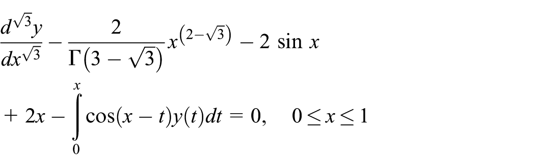
Example 3

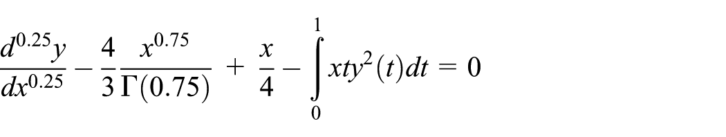
In this example, we consider the nonlinear fractional integro-differential equation

$$\frac{d^{0.75}y}{d{x}^{0.75}}-g\left(x\right)-\underset{0}{\overset{1}{\int }}\mathrm{xt}{y}^2\left(t\right)\mathrm{dt}=0$$

With the initial condition

$$y\left(0\right)=0$$

The exact solution is $y(x)=x^3$ , see Farhood. ¹⁰

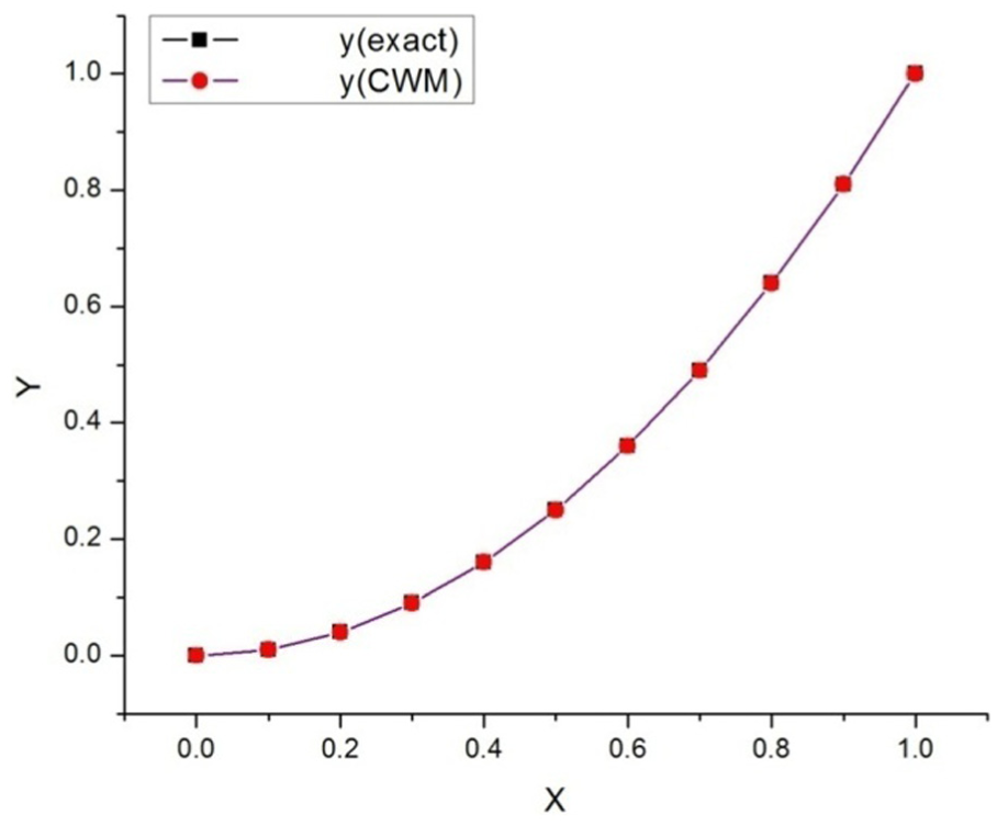
Table 3 displayed the numerical results of example 3 using CWM. The exact solution is represented by y (exact), and approximate solution obtained by CWM is denoted by y (CWM) (Figure 5). Similarly, the errors associated with ADM and CWM is error (ADM) and error (CWM), respectively (Figure 6). The comparison of the errors obtained from ADM and ADM is highlighted. This table shows that the numerical results obtained by CWM are highly accurate than the result of ADM. This method has high degree of accuracy which is the unique feature of this method.

Table 3.

Numerical results for Example 3.

$x_i$	y (exact)	y (CWM)	Error (ADM) 20	Error (CWM)
0.0	0.000	0.00000000000000000001		1.68E−20
0.1	0.001	0.00099999999909354912	2.42E−4	9.06E−13
0.2	0.008	0.00799999999600483058	7.18E−3	3.99E−12
0.3	0.027	0.02699999998967073078	1.65E−3	1.03E−11
0.4	0.064	0.06399999997893393646	2.74E−3	2.10E−11
0.5	0.125	0.12499999996260876951	4.05E−3	3.73E−11
0.6	0.216	0.21599999993949580109	5.57E−3	6.05E−11
0.7	0.343	0.34299999990838754023	7.30E−3	9.16E−11
0.8	0.512	0.51199999986807123419	9.22E−3	1.31E−10
0.9	0.729	0.72899999981733044672	1.13E−2	1.82E−10
1.0	1.000	0.99999999975494604320	1.36E−2	2.45E−10

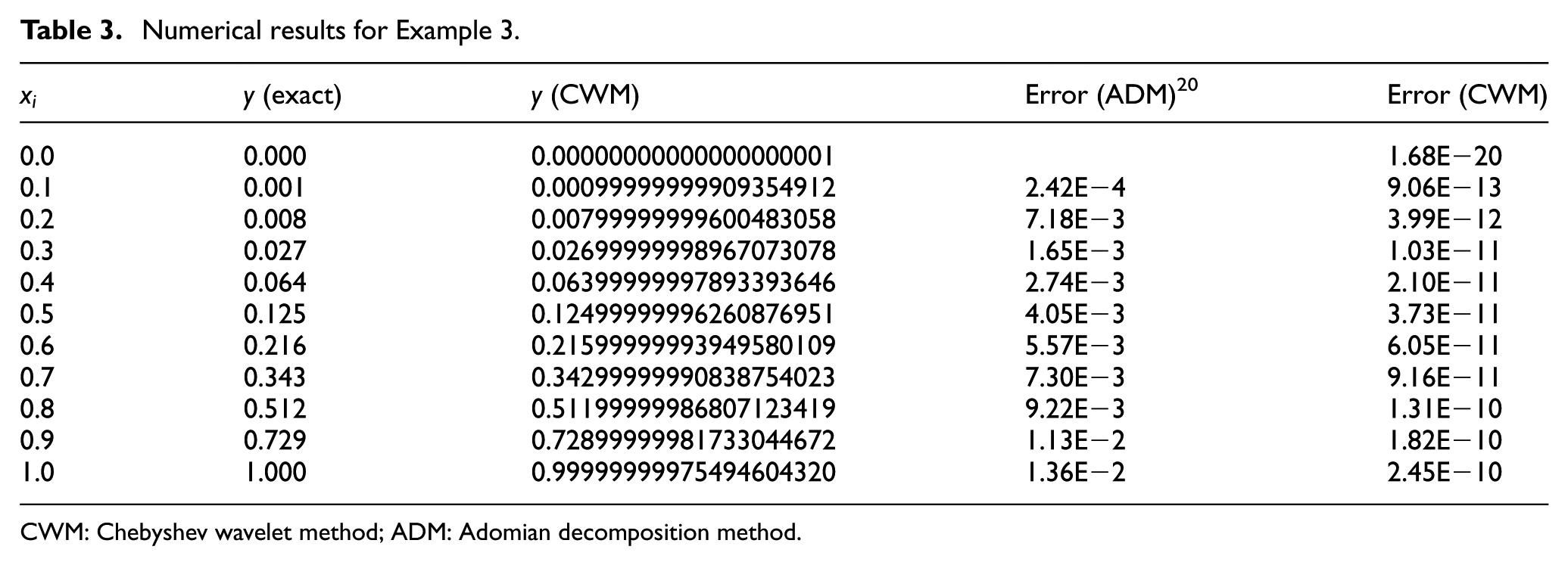
CWM: Chebyshev wavelet method; ADM: Adomian decomposition method.

Figure 5.

The graph of exact solution versus Chebyshev wavelet approximation of Example 3.

Figure 6.

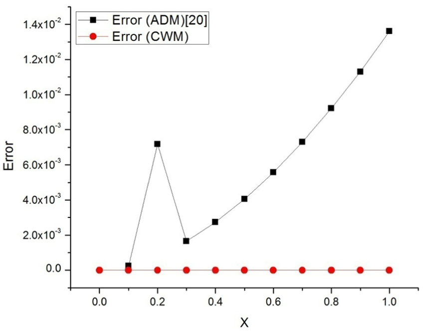
The graph of errors obtained by ADM method and CWM of Example 3.

Example 4

In this example, we consider the nonlinear fractional integro-differential equation

$$\frac{d^{0.25}y}{d{x}^{0.25}}-\frac{4}{3}\frac{x^{0.75}}{\mathrm{\Gamma }(0.75)}+\frac{x}{4}-\underset{0}{\overset{1}{\int }}\mathrm{xt}{y}^2\left(t\right)\mathrm{dt}=0$$

With the initial condition

$$y\left(0\right)=0$$

The exact solution is $y(x)=x$ , see Farhood. ¹⁰

Table 4 shows the numerical results obtained by ADM and the present method CWM. The numerical results obtained by CWM and exact solutions are, respectively, denoted by y (exact) and y (CWM) (Figure 7). The corresponding errors generated by ADM and CWM are denoted by error (ADM) and error (CWM) (Figure 8). The algorithm is applied for $k=1$ and $M=19$ .

Table 4.

The numerical solution of Example 4.

$x_i$	y (exact)	y (CWM)	Error (ADM) 20	Error (CWM)
0.0	0.0	0.00000000000000000001		7.92E−21
0.1	0.1	0.09999999999999999343	1.00E−3	6.57E−18
0.2	0.2	0.19999999999999999638	2.38E−3	3.62E−18
0.3	0.3	0.29999999999999999735	3.95E−3	2.65E−18
0.4	0.4	0.39999999999999999789	5.66E−3	2.11E−18
0.5	0.5	0.49999999999999999815	7.48E−3	1.85E−18
0.6	0.6	0.59999999999999999835	9.39E−3	1.65E−18
0.7	0.7	0.69999999999999999851	1.13E−1	1.49E−18
0.8	0.8	0.79999999999999999860	1.34E−2	1.40E−18
0.9	0.9	0.89999999999999999893	1.56E−2	1.07E−18
1.0	1.0	1.00000000000000005420	1.36E−2	5.42E−17

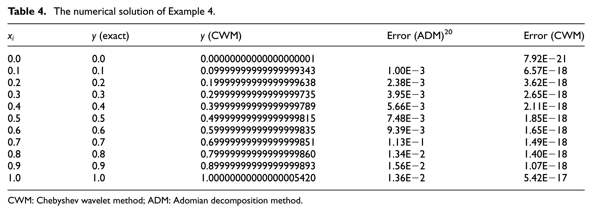
CWM: Chebyshev wavelet method; ADM: Adomian decomposition method.

Figure 7.

The graph of exact solution versus Chebyshev wavelet approximation of Example 4.

Figure 8.

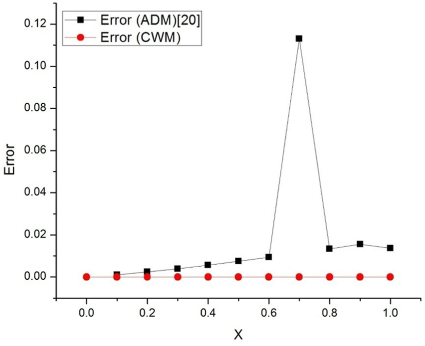
The graph of errors obtained by ADM method and CWM of Example 4.

Conclusion

This work has the capability of introducing an efficient method to solve fractional order Fredholm integro-differential equations. The CWM is implemented to solve these types of integro-differential equations. It is investigated through numerical simulation that the current method has the highest accuracy than any other method in the literature. For future work, we will continue with these techniques for the numerical solution of other high nonlinear integro-differential equations.