
Abstract
This article presents a nonlinear dynamic model of a flexible robotic arm considering nonlinearity from elastic deformation and the effect of gravity. The dynamic model can be decomposed into separate flexible and rigid subsystems. A decomposed dynamic control, including flexible and rigid dynamic controls, is proposed for the controller of the flexible robotic arm. Optimization is used in this flexible dynamic control to obtain the desired trajectory and can deal offline with strong nonlinearity, but it is excessively dependent on the accuracy of the model, so it is not robust enough and has poor disturbance-rejection capabilities. The rigid dynamic control, by contrast, is expected to be sufficiently robust to compensate for uncertain factors. Therefore, a hybrid sliding mode control is proposed to track the desired trajectory and further suppress residual vibration. Additionally, the actual flexible modes are estimated to accurately calculate the component of the proposed controller. This study addresses the theoretical derivation and experimental verification of the proposed controller.
Keywords
Introduction
Flexible robotic arms have the potential advantages of higher payload-to-weight ratio, faster motion, and lower energy consumption. However, they also tend to have vibration problems. Consequently, an accurate model representing actual system behavior and dynamic analysis are required to achieve accurate positioning and vibration suppression.
Edelstein and Rosen 1 proposed two basic modeling approaches for a general flexible multi-body system: the nonlinear continuum approach and the floating frame of reference approach. The latter was used in extensive research on the dynamics of flexible robotic arms. According to studies on flexible robotic arms, the reported approaches that describe elastic deformation can be classified into three groups: The most widely used method is the linear description of deformation;2,3 over the past few decades, several publications have discussed the quadratic deformation approach;4,5 Lee 6 proposed a new description of elastic deformation that synthetically considers the transverse deflection and axial shortening as a vector representing flexible displacement to derive the dynamic model of a one-link flexible beam. This study extends this new approach to a two-link flexible robotic arm, and the effect of gravity should be considered when the elastic and gravitational potential energy is inevitably concerned in the lightweight design of robotic arms.
The derived dynamic model of a flexible robotic arm does not facilitate the feedback-control design as model of a rigid robotic arm because their degrees of freedom to be controlled exceed the number of actuators of flexible robotic arms. To overcome this drawback, a method that reduces the order of the model is required. Several studies have investigated flexible robotic arm in two parts divided from the dynamics. For example, the stable inverse dynamic control 7 calculates the feed-forward torque by assuming the dynamic process to have causal part and noncausal parts; the singular-perturbation approach 8 investigates a flexible system with slow and fast subsystems on the basis of a singularly perturbed model. However, two-part dynamics is derived by pre-multiplying the inversion of the inertia matrix of the full-order dynamics.
Modeling and vibration analysis imply that the flexible robotic arm is a strongly nonlinear system, and a singularity exists in the inversion of the inertia matrix of the full-order dynamics. 9 To avoid the singular inversion of the inertia matrix and decrease the computational difficulty of a complex model with large dimensions, the full-order dynamic equation is decomposed into separate flexible and rigid subsystems. Based on this decomposition of the dynamics into two subsystems, a decomposed dynamic control (DDC), consisting of flexible dynamic control (FDC) and rigid dynamic control (RDC), is proposed. The FDC determines a desired trajectory that can reduce the excitation of the residual vibration, and the RDC tracks the desired trajectory with compensators for uncertain dynamics. 10
In the previous research on FDC, the input shaping technique (IST) and optimization were compared to demonstrate the characteristics of both strategies. IST can determine a desired trajectory on the basis of the principal characters (frequency and damp), 11 but optimization can obtain the desired trajectory based on the total dynamics of flexible structures. Consequently, IST cannot completely remove the residual vibration from strongly nonlinear systems, whereas optimization can completely suppress residual vibration in strong nonlinear systems. 10 Optimization is an offline feed-forward method that deals with nonlinearity and is more economical than the adaptive method. 12 Abe 5 investigated the optimization by minimizing the objective function, which is the maximum elastic displacement of the flexible beam at the end of motion. Benosman and colleagues13,14 proposed backward recursion to optimize the trajectory by minimizing the objective function, which is an elastic energy of the flexible beam at the beginning of motion. In their research, the objective function disregarded the desired states. 15 However, in this study, the objective function in the optimization considers the desired states. In addition, optimization, which is excessively dependent on the accuracy of the model, is not robust and has poor disturbance-rejection capabilities. 10 To compensate for these disadvantages, RDC is expected to possess adequate robustness and disturbance-rejection capabilities to track the desired trajectory with further suppression of residual vibration.
Sliding mode control (SMC) is widely used as a robust approach.16,17 The flexible robotic arm is a typical under-actuated system. Wilson et al. 18 proposed an augmented sliding surface that includes an enhanced term to reject flexible vibration. This method is referred to as augmented sliding mode control (ASMC), where angular actuators (motors) enable each angular joint to rotate and provide damping to suppress flexible vibration. Wang et al. 19 proposed hierarchical sliding mode control (HSMC) for a class of under-actuated systems. The first-level sliding surfaces are conventional, and the second-level sliding surface is augmented.
The augmented sliding surface of an under-actuated system is a hyper plane, consisting of actuated and under-actuated states. The augmented sliding mode surfaces used in published ASMC and HSMC researches have not shown a damping relationship (opposite) between the angular and flexible mode states. This study modifies the augmented sliding surface to design the controller, and the SMC based on the modified augmented sliding surface is termed as hybrid sliding mode control (HySMC) in the RDC. 20
To improve the convergence rate and robustness of the controller, a DDC including optimization and HySMC is proposed to design the controller of the flexible robotic arm. In this controller, the actual flexible modes21,22 are estimated to accurately calculate the nominal components in a dynamic model. An experiment using a two-link flexible robotic arm is performed to verify the theoretical derivation. Figure 1 shows the block diagram of the proposed scheme.

Block diagram of the proposed control.
Modeling the flexible robotic arm
Figure 2 shows the coordinate system of the flexible robotic arm used in this study. The model consists of a rigid link and a flexible beam which is mounted on the second rotational joint with a hub. The O-XY coordinate, denoting the inertial reference frame, is fixed in a slope plane, which forms angle α with the direction of the gravity vector. The o3-x3y3 is the local coordinate system fixed on the hub, where o3 is a fixed point connecting the hub and the flexible beam.
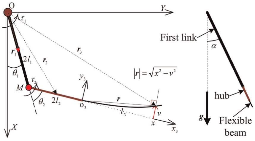
Coordinate system of the flexible robotic arm.
The rigid link has a length of 2l1, θ1 is the rotational angle of joint 1 at the torque τ1, and m1 is the mass of the rigid link. Similarly, the hub has a length of 2l2, θ2 is the rotational angle of joint 2 at the torque τ2, and m2 is the mass of the hub. The motor of joint 1 is assembled on the experimental foundation, and the motor of joint 2, which can be regarded as a point mass M, is embedded at the end of the rigid link.
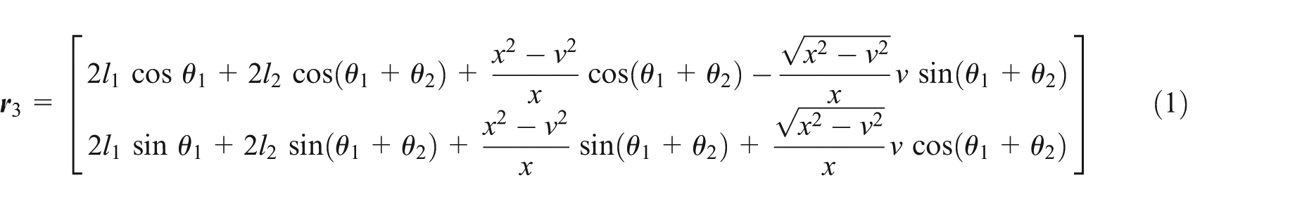
The flexible beam is a homogeneous and isotropic beam with a constant cross section and is modeled as an Euler–Bernoulli beam with fixed-free boundary. The line density and length of the flexible beam are represented by ρ and l3, respectively. The position vectors
In this study, the flexible dynamic model is formulated using the new description of elastic deformation, which is more suitable for modeling in the case of fast motion than the conventional method.9,31 The position vector
The flexible displacement v is expanded in an assumed mode method as follows

where ϕj(x) is the modal function and qj(t) is the modal coordinate. The kinetic energy (K) and the potential energy (P) of the flexible robotic arm are described by the following equations
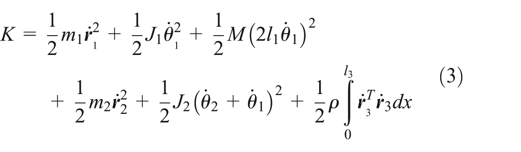
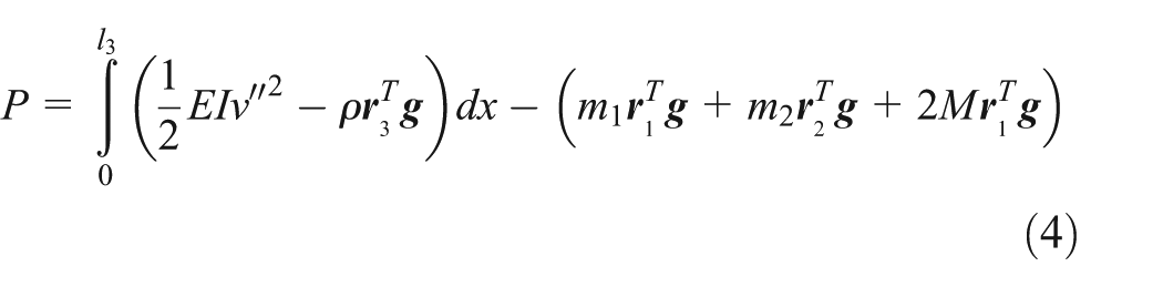
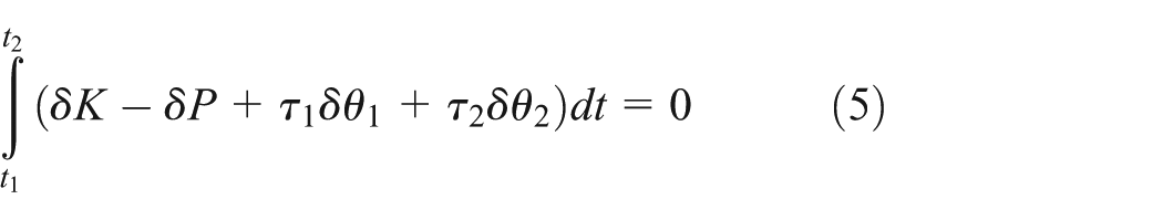
where the mathematical operators · and ′ denote the derivatives with respect to time t and position x, respectively. The dynamic equations of the flexible robotic arm are derived by the following Hamilton’s principle
Then, the nonlinear dynamic equations of the flexible robotic arm are obtained as the following compact form
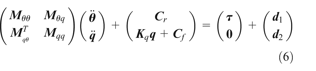
where

where θi is the rotational angle of the ith joint,
This study investigates accurate positioning in joint space and vibration suppression of the flexible manipulator in fast motion, which is denoted as a rotation of 90° within 1 s in the case of considering the high flexibility. Vibration analysis of the flexible robotic arm implies that the dynamic model is strongly nonlinear, and the inversion of its inertia matrix possesses singularity. 9 The inertia matrix of the dynamic model is a function of angular states, modal states, and time. Although the inertia matrix is symmetrical, large deformation results in the rank of the inertia matrix being less than its dimension at some state points, thereby leading to the singularity. If a singularity-related problem exists while applying the dynamic model of the flexible robotic arm, the design on a stable controller becomes difficult. To avoid this difficulty, the dynamic model of the flexible robotic arm is decomposed into a flexible dynamic subsystem (equation (8a)) and a rigid dynamic subsystem (equation (8b)). The two nominal subsystems are described as equations (42)–(47) in Appendix 1, and they are given in the following compact form as
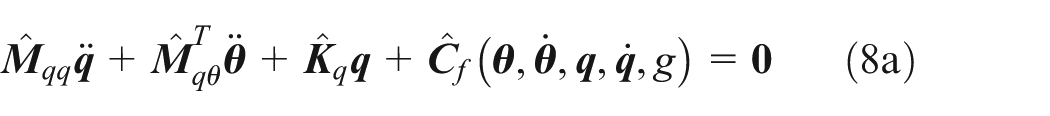
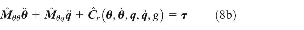
where matrices with ∧ denote their nominal values, which are computable values representing the real values in the models.
In both nominal subsystems, these uncertain inputs from mechanism nonlinearity or actuator faults 24 are not considered, so a robust control strategy is requested to deal with the external disturbance.
Vibration controller design
Based on the decomposition of the full system into two subsystems, a control scheme is proposed for the controller design, which is referred to as DDC, including flexible and RDCs. The FDC involves the development of the desired trajectory based on the flexible dynamic subsystem. The RDC aims to robustly track the desired trajectory and improve the disturbance-rejection capability on the basis of the rigid dynamic subsystem.
Figure 3 shows a block diagram for the DDC. First, optimization is applied to determine the desired trajectory on the basis of the flexible dynamic subsystem. Second, the HySMC is applied to track the desired trajectory with a compensator on the basis of the rigid dynamic subsystem. The proposed FDC 10 shows that the optimization can significantly reduce the residual vibration in the simulation but cannot completely suppress residual vibration in the experiment. This disadvantage results from flexible dynamic uncertainty (Δ f ), which is due to a difference in dynamics between the nominal and actual flexible subsystems. Consequently, RDC presents double tasks in HySMC: 20 the first task enables the accurate and robust tracking of the desired trajectory to compensate for the rigid dynamic uncertainty (Δ r ), and the second task achieves further suppression of residual vibration to compensate for the flexible dynamic uncertainty. Additionally, a nonlinear filter 25 is used to estimate the actual modal variables.

Diagram of control schemes of the plant.
Optimization
The task of optimization involves obtaining the desired trajectories (
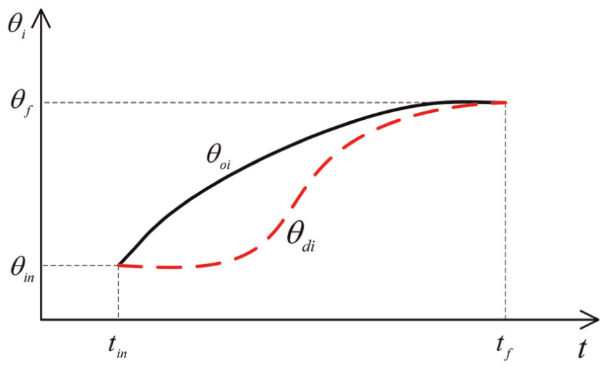
Schematic diagram of the original and desired trajectories.
The desired trajectory is where the initial and final positions are the same as the values of the original trajectory (
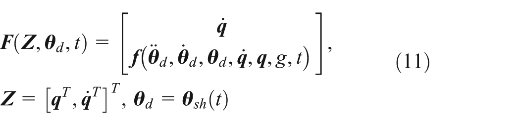
Optimization is based on the flexible dynamic subsystem (equation (8a)). In this study, the first link is a rigid body and the flexible beam is fixed on the second joint with a hub. Therefore, two angular trajectories are optimized to reduce residual vibration of the flexible beam. To describe the process, we transform the flexible dynamic subsystem as follows

where
For optimization, the angular functions (angular position, velocity, and acceleration) are the control inputs. The task of optimization is to determine the desired control input that can reduce excited vibration. The state equation with the desired control input can be expressed as follows

where
Here,

where bij is the constant coefficient and tin and tf are the initial and final times of motion, respectively, and are shown in Figure 4.
The boundary conditions of the shaped function are given as follows

Six boundary conditions exist for each shaped trajectory, and assuming a shaped trajectory with more than six terms (N > 5) in the optimization is reasonable. The first six coefficients can be expressed with the last n coefficients, where n = N − 5. The series of the last n independent variables is given as a vector

Substituting equations (12)–(14) into equation (10), we can obtain a new state equation with variable

where
The state variable
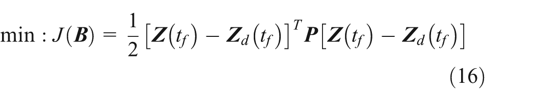
where
The desired trajectories are a map of the design variables, and the solution for the design variables is equivalent to that for the desired trajectories. After obtaining the desired trajectories, a robust control system is designed to track the desired trajectories, and this system is explained in the next section.
HySMC
In this section, the control module is designed on the basis of the rigid dynamic subsystem (equation (8b)). This subsystem can be transformed into a compact form as follows

where
Equation (17) denotes that the rigid dynamic subsystem is a typical under-actuated system, which means that the motors of the joints not only drive the angular rotation but also suppress the flexible vibration if no other type actuators are used to suppress vibration except for motors. To design the control module, the rigid dynamic uncertainty is assumed to satisfy the matching conditions 27 and the uncertainty is expressed as

Here, Ni is the uncertain boundary of the nonlinear force and Ri is the component of the nonlinear vector

The subscript i = 1, 2;

To enable the rotational motion of the flexible robotic arm to further suppress the vibration in RDC, a dissipative structure is expected to be present in the control module. Based on this principle, the augmented sliding surfaces are composed of the joint variables (

where
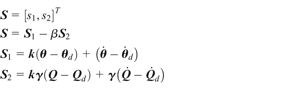
where

Here, β is the damping coefficient given as a positive constant.
Using the equivalent control principle and substituting equation (17) into the differential function (
In addition to the equivalent control terms, the control module should include a few variable structure terms. In the design of variable structure terms, the reaching law is defined as follows

Here,

where

The variable structure control input can be obtained as follows

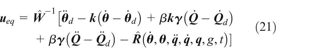
The variable structure terms are uncoupled and are derived by defining the reaching law (22). The control module includes the equivalent control (21) and variable structure control (24), and the total control law of the control module is expressed as follows

To reduce the chattering of the control system, sign function sgn(s) in the proposed control module is replaced by a continuous, hyperbolic tangent function tanh(s). 16
To further suppress the residual vibration, flexible deformation is measured by strain gauges. In the proposed controller, the flexible modes (
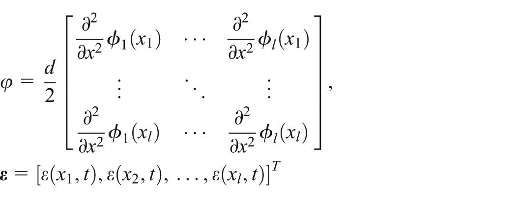
The mathematical equation relating the flexible displacement and the strain in a location at the flexible beam is expressed as follows

where d is the thickness of the flexible beam; substituting equation (2) into equation (26), the following equation is obtained

If l strain gauges are attached at different points along the flexible beam, namely, x1, x2,…,

where
To determine vector


The detailed derivation of the inequality of Lyapunov’s stable condition is listed as follows

An equivalent inequality that satisfies the above stable condition is obtained as follows

where i = 1, 2. If an appropriate positive constant is inserted into the right side of the inequality, the above inequality can be transformed into an equality, which is described as follows

where ζi > 0, i = 1, 2. The set of equations can be rewritten as a matrix equation

where

Based on the definition (23), parameter

Here,
Experimental results
To verify the validity of the proposed controller, this section discusses the experiment wherein a flexible stainless steel beam with a constant cross section is used. The mechanical parameters of the flexible robotic arm are as follows: The width and thickness of flexible beam are 0.037 and 0.500 × 10⁻³ m, respectively. The line density and length of the flexible beam are ρ = 0.142 kg/m and l3 = 0.400 m, respectively. Young’s modulus and moment of inertia of the flexible beam are E = 200 GPa and I = 5.40 × 10⁻¹³ m4, respectively. The mass of the second joint is M = 0.600 kg, and the lengths of the rigid link and hub are 2l1 = 0.300 m and 2l2 = 0.070 m, respectively. The angle of the slope is α = π/6.
Before the real-time tracking control, a desired trajectory is determined using an optimization module, which runs offline. The original trajectories for the two joints in the maneuver are defined as follows
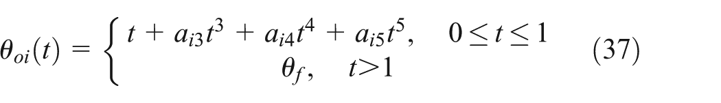
where ai3 = 10θf − 6, ai4 = −15θf + 8, and ai5 = 6θf − 3, i = 1, 2.
The desired trajectories are the functions of
Optimization results of the design variable

In this experiment, the proposed controller is applied to the two-link flexible robotic arm shown in Figure 5. The flexible robotic arm is composed of a rigid link, flexible beam, and two rotational joints. The stator of the first rotational joint is mounted on the experimental foundation, and the stator of the second rotational joint is embedded at the end of the first link. The first link is fixed on the rotator of the first joint, and the flexible beam is connected to the rotator of the second joint with a hub.

Experimental setup of the flexible robotic arm.
The first rotational joint is an AC servo motor (SGMJV01ADAH701, 100 W) and the second rotational joint is a relatively small AC servo motor (SGMJVA5ADAHC01, 50 W). A real-time processor DSP7100 (Mtt Corp.) is used to rapidly deal with the algorithm. The DSP7100 has a 32-bit counter that computes angular positions and velocities by obtaining the encoder signal from the servo motors. A total of two strain gauges (l = 2) are pasted on the flexible beam to measure the strains of two locations (in the local frame, x1 = 0.05 m and x2 = 0.1 m). The strain signals are amplified by a dynamic strain amplifier DC204Ra (Tokyo Sokki Kenkyujo Co. Ltd.). These angular and strain signals (θ and q) are used in feedback control. The data for the control program are written on a PC, and it is downloaded into DSP by an Ethernet cable; the experimental results are also obtained through the PC. Additionally, a serial RS232 port is used to modify the communication protocol between the DSP and the PC. The configuration of the experimental system is shown in Figure 6.
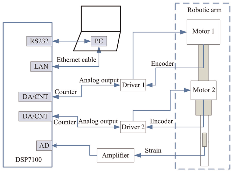
Configuration of the experimental system.
In this experiment, a friction compensate function 28 is used to reduce external uncertainty, and the mathematical model of friction compensation is defined as follows

where µsi and µci are the unknown static and Coulomb friction, respectively. The unknown friction functions are replaced by a boundary value where |µsi| ≤ usi and |µci| ≤ uci. λi is a switching function, which is defined as follows

where ωi is the critical constant of the angular velocity that characterizes the Stribeck effect, 29 and the subscript i represents the friction working on the ith joint. In this experiment, the critical constant is assumed to be a positive infinitesimal.
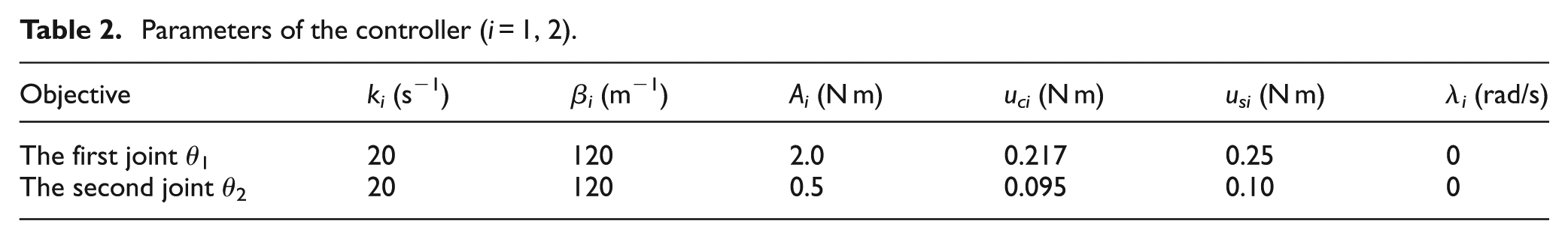
The original and desired trajectories are tracked to compare the residual vibration resulting from the respective excitement in the experiment (β = 0). Additionally, the desired trajectories are tracked with a flexible dynamic compensator to further suppress the residual vibration (β = 120). The parameters of the proposed controller, which are determined by trial-and-error during the experiment, are given in Table 2.
Parameters of the controller (i = 1, 2).
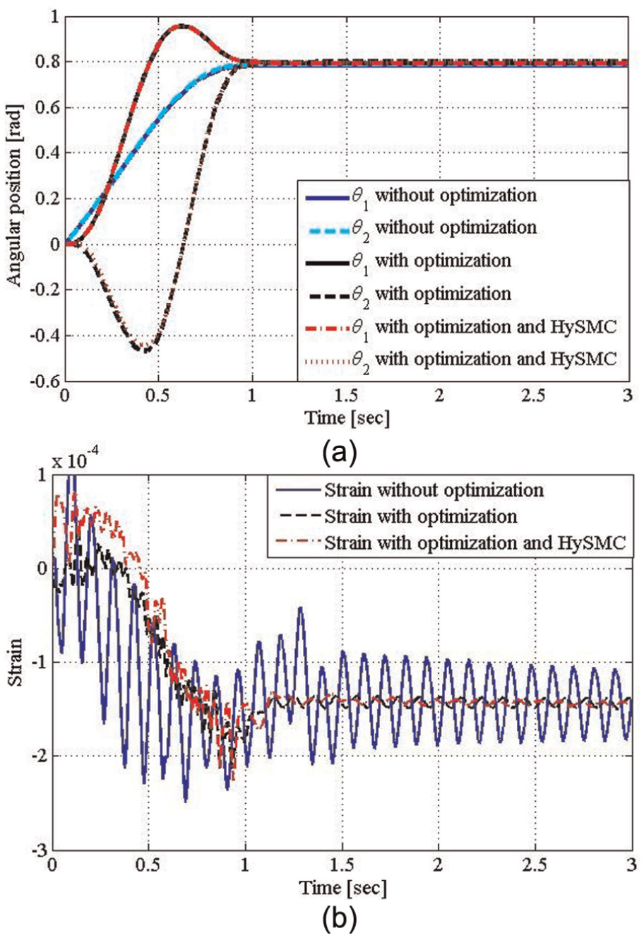
Similarly, this experiment is performed by two maneuvers. In the first maneuver, the final angular positions of the two joints are θf = π/2, and the flexible beam is expected to be located in the vertical plane after the rotation. In the second maneuver, the final angular positions of both joints are θf = π/4, and the flexible beam is expected to be positioned in the horizontal plane after the rotation. Figure 7 shows the experimental results for the case in which the flexible beam is expected to be located in the vertical plane. Figure 8 shows the experimental results for the case in which the flexible beam is expected to be located in the horizontal plane. In the former case, the residual vibration of the flexible beam is symmetrical about zero after the rotational motion. In the latter case, by contrast, the residual vibration of the flexible beam is symmetrical around a statically deformed position after the rotational motion. The static deformation appears due to the effect of gravity.

Experimental results where the flexible beam is located in the vertical plane (θf = π/2,
Experimental results where the flexible beam is located in the horizontal plane (θf = π/4,
The tracked trajectories are shown in Figures 7(a) and 8(a). The first link is the rigid body, and the flexible dynamic compensator does not function during the tracking of the first joint. Therefore, the results show that the red dashed–dotted line roughly overlaps with the black solid line. Given that the second link is a flexible beam and the flexible dynamic compensator is used in the feedback control to further suppress the residual vibration, the results show that the red dotted line slightly deviates from the black dashed line in Figures 7(a) and 8(a). This minute deviation indicates the activity of the flexible dynamic compensator.
To show the flexible dynamic compensation, the tracking errors of trajectories are defined as

where θoe and θos denote the original trajectories in experiment and simulation, respectively; θde and θds denote the desired trajectories in experiment and simulation, respectively; θdhe denotes the desired trajectory tracked by HySMC in experiment; and the subscript i denotes the values of the ith joint.
The tracking errors in both cases are shown in Figures 9 and 10. The original errors (Δθoi) of the second joint are smaller than the original errors of the first joint; this point implies that the original trajectories of the second joint are tracked more effectively than original trajectories of the first joint. The desired errors (Δθdi) are almost the same as the hybrid errors (Δθdhi) in the first joint because the first joint does not consider the compensation for flexible vibration, but the desired errors are significantly different from the hybrid errors in the second joint due to the effects from the flexible vibration.

Errors of flexible beam located in a vertical position (θf = π/2,

Errors of flexible beam located in a horizontal position (θf = π/4,
Figures 7(b) and 8(b) show these strains at tip position of flexible beam on the action of three different trajectories. When the original trajectories of the two joints are tracked (without optimization), a significant residual vibration occurs after the rotational motion. When the optimized trajectories are tracked, although the residual vibration is relatively smaller, it still exists. If the optimized trajectories are tracked with a flexible dynamic compensator (HySMC), the residual vibration is further suppressed; however, larger residual vibrations occur in Figure 8(b) than that in Figure 7(b) after 1 s because of the effect of gravity. When handling the links with high flexibility, there would be limitations to suppress vibration in this case.
To disclose the convergence rate of vibration suppression, a comparison between these relative errors at the main points of flexible beam in this study (red line) and in the literature 18 is provided in Table 3, where these relative errors are defined as

where er and e are relative error and error at arbitrary time, respectively, and ε and εd represent that the strain at arbitrary time and its desired value, respectively.
Comparison between errors relative to the desired value.
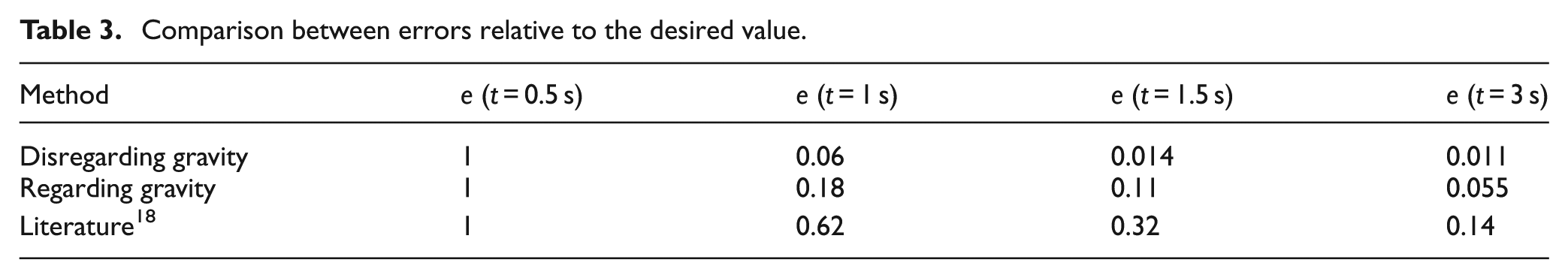
If the relative error is <0.1, the flexible vibration is deemed as convergence; as we know from Table 3, the settling time of the vibration disregarding gravity occurs in 1 s, and that regarding gravity occurs about 1.5 s, while the settling time of vibration in the literature 18 exceeds 3 s.
According to the comparison with reported studies on SMC, such as literature, 18 we can know that this study combining HySMC with optimization possesses higher convergence rate of vibration control.
The experimental results verify that the DDC is a robust method to deal with the complex system considering the nonlinearity and effect of gravity but short of the sensitivity for error resolution. The accurate modeling of mechanism nonlinearity and even actuator faults 30 is expected to implement exact and reliable control in future work.
Conclusion
This study adopted a new description of elastic deformation on the flexible beam and considered the effect of gravity to formulate a dynamic equation for a flexible robotic arm. An analysis of vibrations using the proposed dynamic equation indicated that the inversion of the inertia matrix resulted in singularity at some state points. To avoid the singularity problem in torque computed components of controller, the dynamics equation was decomposed into flexible and rigid dynamic subsystems. Based on the decomposition, a DDC was proposed to design the controller of the flexible robotic arm.
The DDC consists of an offline optimization and HySMC. The optimization focuses on obtaining the desired trajectories by adopting modified objective function and forward recursion, whereas the HySMC involves tracking the desired trajectories and increases vibration suppression. Optimization can deal with strong nonlinearity in dynamics, but it is not robust and has poor disturbance-rejection capabilities, so it is excessively dependent on the accuracy of the dynamic model. Therefore, the proposed DDC combined HySMC with optimization to improve the properties of the controller for flexible robotic arms.
The experimental results verified the validity of the proposed controller and implied certain limitations on the system with high flexibility when considering the effect of gravity. In addition, the practical applications of the proposed results to the lightweight design on industrial robots should be investigated, and the definition of Markov chains, 23 the modeling of actuator fault, 24 and reliable control of robotics with Markovian jumping actuator faults 30 are also part of our future works.
Footnotes
Appendix 1
First, the flexible dynamics with the first two modes are represented by
where γj and βj are the coefficients of the linear or nonlinear terms, and φ = g cos α. These coefficients are described as follows
where φi(x) is modal function of flexible beam in the fixed-free case.
In addition, the rigid dynamics with two angular inputs are expressed as
Acknowledgements
The authors are grateful to the Editor-in-Chief, the Associate Editor, and anonymous reviewers for their constructive comments based on which the presentation of this article has been greatly improved.
Academic Editor: Hamid Karimi
Declaration of conflicting interests
The author(s) declared no potential conflicts of interest with respect to the research, authorship, and/or publication of this article.
Funding
The author(s) disclosed receipt of the following financial support for the research, authorship, and/or publication of this article: This study was supported by the National Natural Science Foundation of China under grant 11202153 and the Scientific Research Foundation for the Returned Overseas Chinese Scholars, State Education Ministry under grant 2013-693.