
Abstract
This article proposed a novel approach for the dynamic modeling and controller design of a passive-wheel snake robot based on Udwadia–Kalaba theory. Compared to common methods, this approach is easily processed for many-degree-of-freedom snake robot. The desired trajectory is easily modeled as a trajectory constraint, and the nonholonomic constraints from the passive wheels’ lateral velocity are also easily handled using Udwadia–Kalaba theory. Besides the proposed equation of motion is analytical, no approximation or linearization as well as extra variables such as Lagrangian multiplier is needed as common methods usually do. The servo joint constraint forces are precisely calculated by solving Udwadia–Kalaba equation, and no complicated control structure design is needed as common control methods always do especially for under-actuated mechanical systems. This article provides a novel dynamic modeling and controller design approach for the passive-wheel snake robot in a new perspective. The theoretical analysis and simulation verify the proposed approach. The trajectory has good incidence with the designed one, and the real-time joint forces are also conveniently acquired.
Keywords
Introduction
As a type of bionic robots, the snake robot is drawing attention in recent years. The snake robot can do a number of works such as environment detection, resource prospecting, and pipeline maintenance, which is difficult or dangerous for human beings to process. In the above application fields, the snake is usually controlled to fulfill a desired motion.
Because of the nonlinear, nonholonomic, and under-actuated characteristics of the passive-wheel snake system, the modeling and control is always difficult to handle. On one hand, the modeling quality of the snake system has significant influence on the control performance of the snake. As a many-degree-of-freedom mechanical system, the dynamic modeling of the passive-wheel snake robot is complicated and difficult to process using classical dynamic theory such as Newton equation and Lagrangian equation which are mostly used in the snake’s modeling. Moreover, approximation and linearization are always used when using common methods to model the snake which detects the modeling accuracy. Besides, it is always not easy to model the passive wheels’ nonholonomic constraints. Currently, there are mainly two ways to handle these constraints. First, the passive wheels’ constraints are modeled by a “geometry equality method,” that is, the nonholonomic constraint imposed on the snake body. Second, one can also use the “force equality method” to model these constraints, in which the passive wheel is simulated by an infinite lateral force and a zero-longitudinal force. However, most of the current dynamic theories show difficulty when dealing with such constraints.
On the other hand, as an under-actuated mechanical system, the trajectory tracking control of the snake robot is always difficult and complicated to handle. Commonly, common methods always make assumptions of the model which detects the control accuracy. Moreover, extra procedure variables, such as Lagrangian multiplier, make the controller design difficult and complex. Besides, the modified controller structure such as added visual sensors which is processed in the controller design procedure when using common control methods also makes the controller design a heavy task.
Many researchers have done much work on the dynamic modeling and controller design of the snake robot. Krishnaprasad and Tsakiris 1 and Kelly and Murray 2 modeled the passive-wheel snake robot using differential geometry method and discussed the controllability of the proposed model. Ostrowski 3 and Ostrowski and Burdick 4 provide the dynamic model of the snake and simplified it considering the symmetry of group. Prautsch and Mita 5 modeled a plat snake robot using Lagrangian equation and studied its tracking control performance based on Lyapunov theory. Date et al.,6,7 Watanabe et al.,8,9 Hicks and Ito, 10 and Toyoshima et al. 11 modeled the snake and studied the optimized torque control of the system on the basis of classical dynamic theories. Lijieback et al.12–14 achieved the trajectory tracking controller design for the snake robot. Alamir et al. 15 and El Rafei et al. 16 designed feedback control scheme and sliding mode control scheme for snake-like eel robot. Guo et al.17,18 utilized the fiber bundle theory to realize the snake’s modeling and researched the optimal torque control of the snake.
However, all the above methods are mathematically difficult and complicated, either making approximation or linearization of the dynamic model or making a modified structure of the controller, which detects the modeling quality and the control performance. In this article, we propose a novel approach of the modeling and controller design of the passive-wheel snake robot on the basis of the Udwadia–Kalaba theory. Compared to common methods, this approach provides analytical equation of motion of the snake system, in which the nonholonomic wheel constraints are easily modeled. Besides, this approach is easy to handle, especially applicable for the modeling of many-degree-of-freedom snake systems, without extra process variables such as Lagrangian multiplier. Based on the proposed Udwadia–Kalaba fundamental equation of motion, the controller is also designed handily without any extra structures of the controller. The servo constraint forces of the joints are acquired exactly by solving the Udwadia–Kalaba equation, and the snake can move exactly in excellent coincident with the desired trajectory.
Classical dynamic theories for constraint mechanical system are derived on the basis of d’Alembert’s principle and virtual displacement principle, such as Newton–Euler equation, Lagrangian equation, Boltzmann equation, Maggie equation, and Hamel equation.19–25 Because of the assumptions in the above theory, as well as the conditions for many-degree-of-freedom mechanical systems, the applications of the classical dynamic theory turn out not optimistic. Besides, the lack of flexibility of the classical dynamic theories makes it complicated and difficult to model a practical mechanical system, especially for a complex mechanical system with different types of constraints.
On the basis of former researches, Udwadia and colleagues26–31 provided fundamental equation of motion of constraint mechanical systems. Compared to classical dynamic theories, the equation of motion is easily acquired mainly by three steps, without any other variables such as Lagrangian multiplier in Lagrangian equation, which is handy to process. Moreover, the equation is in more exact analytical form, because of no linearization or application in the derivation. Besides, this approach can deal with ideal or nonideal constraints and holonomic or nonholonomic constraints, applicable also for over-actuated or under-actuated systems. Moreover, the number of coordinates turns out less important, as long as the constraint equations are consistent and the mass matrix is positive definite. The Udwadia–Kalaba theory brings a new perspective for the trajectory tracking problem.
In analytical dynamics, the trajectory tracking control problem is also defined as a problem of servo constraint control. Udwadia and colleagues32–34 first made a preliminary research in the field of nonlinear mechanical systems using servo constraint control method. Chen35–38 achieved the systematical servo constraint controller design of mechanical systems based on Udwadia’s research and also studied servo constraint problem, indicating that based on Maggi equation, the required constraint inputs can be acquired by servo control. Schutte 39 studied the modeling and control problem of nonholonomic mechanical systems when using Udwadia–Kalaba equation and designed nonlinear feedback controllers for such types of mechanical system, and Bajodah et al. 40 focused on the mathematical calculation problems in servo control solution when using Udwadia–Kalaba equation, essential for the practical application of this equation. Chen et al.41–43 also researched on the adaptive robust control of uncertain mechanical systems on the basis of Udwadia–Kalaba theory.
It is useful to handle the dynamic modeling and control problem based on Udwadia–Kalaba theory. First, the modeling is easy to process, consists of mainly three steps, especially for the modeling of a many-degree-of-freedom snake robot. Not only the more accurate analytical equation of motion can be acquired, without using any extra process variables such as Lagrangian multiplier, but also the nonholonomic lateral velocity constraints can also be handily modeled. The desired trajectory is treated as a constraint named trajectory constraint in this approach, which is conveniently modeled in the Udwadia–Kalaba equation. Second, based on the proposed dynamic model, the controller design can be derived directly, no linearization or approximation of the model or modification of the controller is needed such as visual sensors as common methods usually do, especially for the under-actuated nonholonomic passive-wheel snake robot system. The real-time joint constraint forces can be acquired easily by solving Udwadia–Kalaba equation, which is efficient for the snake’s exact motion control.
This article proposed a novel approach for the dynamic modeling and controller design of the passive-wheel snake robot based on Udwadia–Kalaba theory. The nonholonomic wheel constraints are handily modeled in the Udwadia–Kalaba fundamental equation of motion. This approach makes the modeling process of the many-degree-of-freedom snake robot system simplified largely by mainly three steps, without any extra process variables. The equation of motion is analytical, without any simplification of the system as common methods usually do, which is significant for the motion performance of the snake. The controller is also designed on the basis on the proposed dynamic model. The servo joint constraint forces of the snake are acquired exactly by solving the equation of motion, and the calculated trajectory is of good coincident with the desired one. The controller is easy to achieve because of no extra structure design of the control system, which is always complicated when using common methods where extra structures such as visual sensors are essential.
Dynamics of Udwadia–Kalaba theory
First consider the unconstrained mechanical system with the n generalized coordinates, denoted by

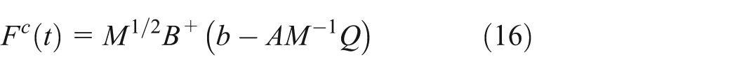
where
The generalized acceleration of the unconstrained system at time t, which is defined by

Second, constraints imposed on the system are considered. The constrained system is assumed to be subjected to h holonomic constraints in the form of

and

The constraint equations must be consistent so that we do not care whether the constraints are linearly independent or not in this article.
The constraint matrix equation can be acquired by differentiating holonomic constraints (equation (3)) twice and nonholonomic constraints (equation (4)) once with respect to time t, respectively, and is given by

where
Remark 1
As we know, constraint equation used in classical dynamics such as Lagrangian equation, Maggi equation, and Gibbs and Appell equation is either in the zero-order or first-order form. While the constraint equation of Udwadia–Kalaba equation is in a second-order form, which is more flexible for manipulating the equations. 37 The second-order constraints are the most suitable form for further dynamic analysis. The second-order constraint is useful because the constraint equation is linear in acceleration. Using the second-order constraints of fundamental equation of motion, one can handily analyze discontinuous acceleration problems. Furthermore, the second-order form constraints can also be used to prove the Gauss’ principle.
By combining the unconstrained equation of motion (1) and the constraint equation (5), the analytical Udwadia–Kalaba equation of motion of the constrained mechanical system is finally acquired. Additional generalized constraint forces resulting from the constraints should be imposed on the system. The actual equation of motion of the constrained system can thus be written as

where
In Lagrangian dynamics,

where
Equation (6) is more general which is applicable for system with ideal constraints as well as nonideal constraints.

which is the extended Lagrange’s form of d’Alembert’s principle. The work done by the ideal constraint force

while the work done by nonideal constraint force is

Udwadia and Kalaba have proved that the ideal constraint force can be given by

and the nonideal constraint force takes the form of
where
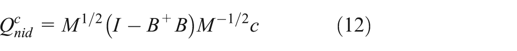
From equations (6), (7), (11), and (12), the analytical equation of motion of general constrained mechanical system can be given by
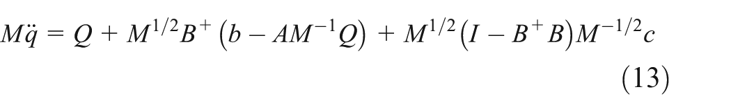
where the vector c is determined by the mechanician and can be obtained by observation or experimentation.
Equation (13) is called the Udwadia–Kalaba fundamental equation of motion. When c equals zero, equation (12) reduces to d’Alembert’s principle, which means the total work done under virtual displacement is zero from equation (8). For an ideal constrained system, we thus have

and the equation of motion of the ideal constrained system is

Therefore, the required additional constraint force
Remark 2

and if the unconstrained acceleration

Remark 3
For equation (13), if the mass matrix M is singular, the Udwadia–Phohomsiri 27 equation should be used instead of Udwadia–Kalaba 29 equation to acquire the equation of motion of the constrained system, and the equation of motion becomes

The above equation is valid when the matrix [M|A]T has full rank. 27
Dynamics of the snake
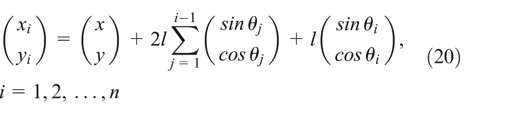
As is shown in Figure 1, we design the earth fixed frame I to study the modeling and control of the n-link passive-snake robot which moves on a flat ground. The earth fixed frame

Modeling of the snake.
The lateral velocity of each wheel equals to be zero to mimic the friction characteristic of snake’s abdomen. For an n-link snake robot, the relationship between
Differentiating the above equation with respect to time t once, we obtain

The nonholonomic lateral velocity constraints can be written as

Combining equation (21) and (22), we have

From equation (5), differentiating equation (23) with respect to time t once, we obtain equation (24)

The nonholonomic constraints can thus be written in the matrix form, given by

where

where
Now, we derive the equation of motion of the snake without the lateral velocity constraints using Lagrangian equation. The system’s kinetic energy can be given by

From the Lagrangian equation, the equation of motion of system without lateral velocity constraints can be given by

Substituting equation (21) into equation (27), we have

where

where

Generally, the head of the snake is designed to track a desired trajectory to accomplish a certain tracking task. The problem of constrained motion in analytical dynamics can be reframed as a trajectory tracking control problem, based on Udwadia–Kalaba theory. And the desired trajectories are treated as constraints named trajectory tracking constraints in Udwadia–Kalaba theory. The desired trajectory, say, the trajectory tracking constraint, can be written in the form of constant equation (5), and the servo constraint force
The desired trajectory tracking constraints

where
Now, we convert the constraints into the second-order form. Differentiating constraint equation (30) with respect to t yields

where

and

The second-order form of the constraints can be rewritten as

or in the matrix form

where
Remark 4
Similarly, if a constraint equation is given in the zero-order form, differentiate it with respect to t twice, and if a constraint equation has one-order form, differentiate it with respect to t once, and the second-order form constraint equations can thus be acquired. All one needs to do is to prescribe a desirable system constraint and then convert it to a second-order form.
Remark 5
In fact, the second-order form constraint equation (35) is a very general form. It includes typical constraints as illustrated by Rosenberg 19 (1997). It also includes a number of standard control problems such as stabilization, trajectory following, and optimality.36,37 The trajectory tracking constraint is just one of these constraints above.
Combining equations (25) and (35), the constraint of the snake system can thus be written as

where

Controller design
The joint constraint force
The joint servo constraint force

the servo joint constraint force can thus be solved by

where the superscript “+” denotes the Moore–Penrose generalized inverse.
Remark 6
One should determine the servo structure by choosing D to obtain
The complete snake system control diagram is summarized in Figure 2, where

Control system of the snake robot.
The initial conditions
According to the Lyapunov stability theory, the following differential equation can be constructed

where
This equilibrium point is globally asymptotically stable.
Usually, numerous systems fulfilling the above two conditions can be constructed, such as

these constraints can be modified as

with
Remark 7
In reality, there are a number of uncertainties in practical systems, such as the initial positions, the external disturbances, and the parameter variations. The constraint stability method 41 is useful for handling these uncertainties to achieve the exact adaptive robustness control of the system.
Based on Udwadia–Kalaba equation, the control input (38) can be rewritten as

where
Simulation
We start with the dynamic modeling and the controller design of a three-link snake robot using the proposed approach derived from Udwadia–Kalaba theory.
For n = 3, from equation (20–25), we have the lateral velocity constraints

where

From equations (26)–(29), the dynamic equation of motion of the three-link snake robot without lateral velocity constraints can be given by

where
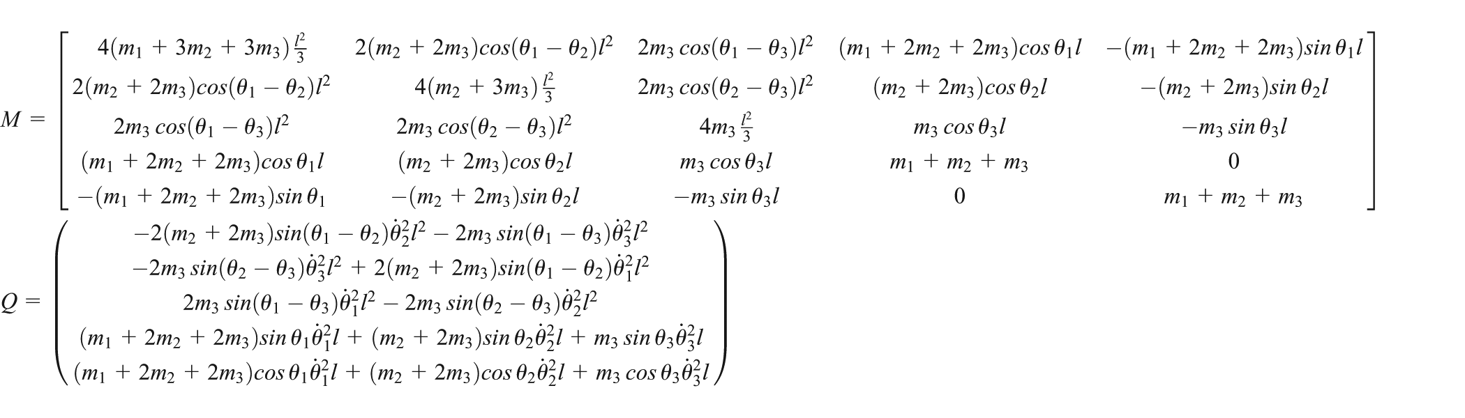
and

where the angle converting matrix
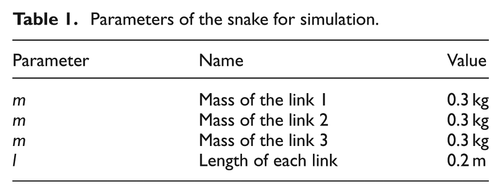
Based on equations (44) and (45), the servo joint constraint forces can be acquired by solving equation (38). Table 1 shows the parameter values of the snake for simulation.
Parameters of the snake for simulation.
Simulation 1
We assume the snake’s head to track a circle to achieve a certain tracking task. The desired trajectory

Differentiating constraint equation (46) with respect to t once and twice, respectively, yields
and

In this article, the initial conditions satisfy the desired trajectory tracking constraint equations for the simplification of simulation.
The initial conditions containing initial displacement and velocity of the snake can be calculated by letting
Initial conditions for simulation 1.

We use ode45 integrator in MATLAB to process the simulation of the proposed approach. The simulation time is 15 s. Figure 3 shows the calculated trajectory of the snake’s head as functions of time t, where x and y represent the displacements of x-axis and y-axis of the head, respectively. We can see clearly from Figure 3 that the position is well coincident with the desired motion (46). By solving equation of motion (38), the required real-time servo joint forces are acquired as Figure 4 describes.
Calculated position of the snake’s head versus time (circle trajectory).
Calculated required servo joint forces versus time (circle trajectory).
A more detailed tracking performance of the numerical errors of head’s position as functions of time is given in Figure 5. From Figure 5, we can see that the error between the calculated position and the desired, say, the trajectory tracking constraint equations (46), is small enough. Specifically, the trajectory tracking error is given by

Position error of the snake’s head versus time: (a) position error of x direction versus time and (b) position error of y direction versus time (circle trajectory).
Figure 6 shows a much more intuitive description of the trajectory tracking performance. Figure 6 shows the calculated and desired trajectory of the snake’s head. We can also conclude that the tracking error is really small that the two trajectories have a good coincidence.

Calculated/desired trajectory of the snake’s head (circle trajectory).
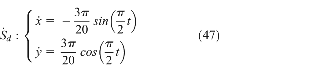
Simulation 2
We also assume the snake’s head to track a sine curve to achieve a certain tracking task, given by
Differentiating (49) with respect to t once and twice, respectively, we have
and
The initial conditions satisfying the constraints are given in Table 3.
Initial conditions for simulation 2.

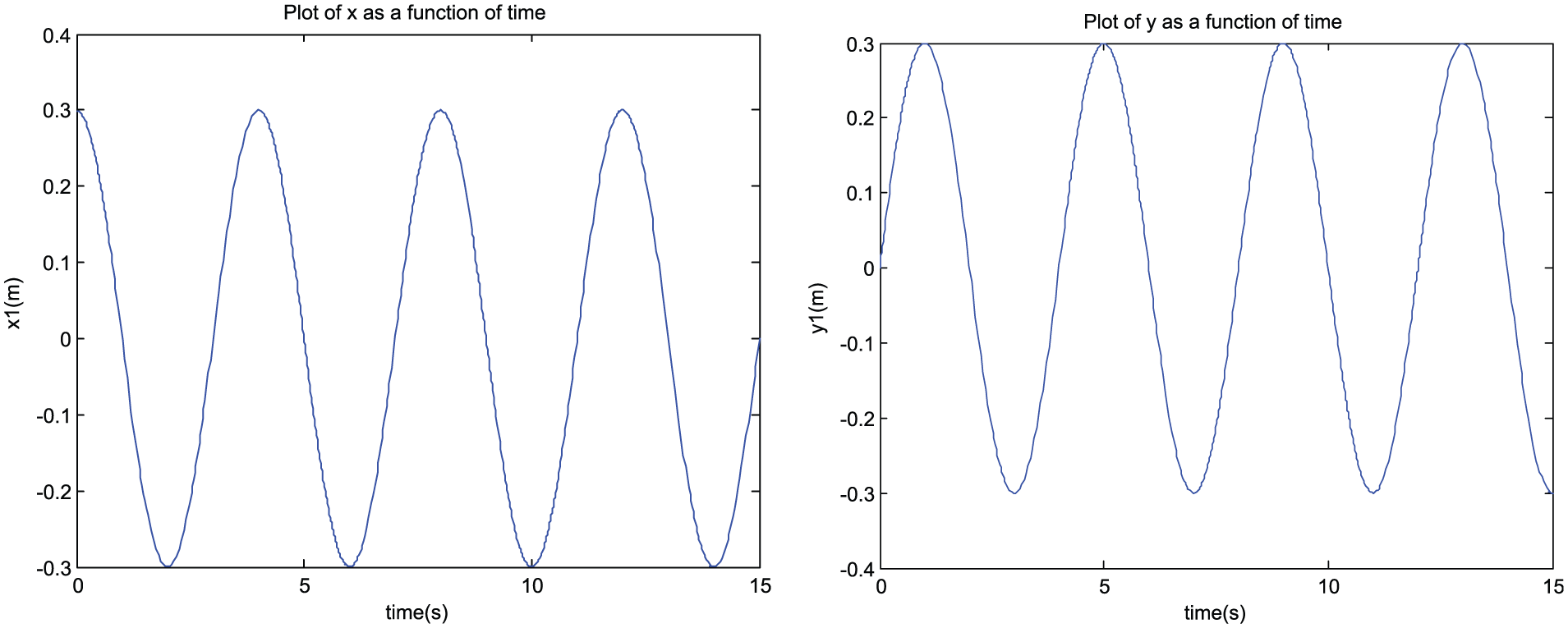
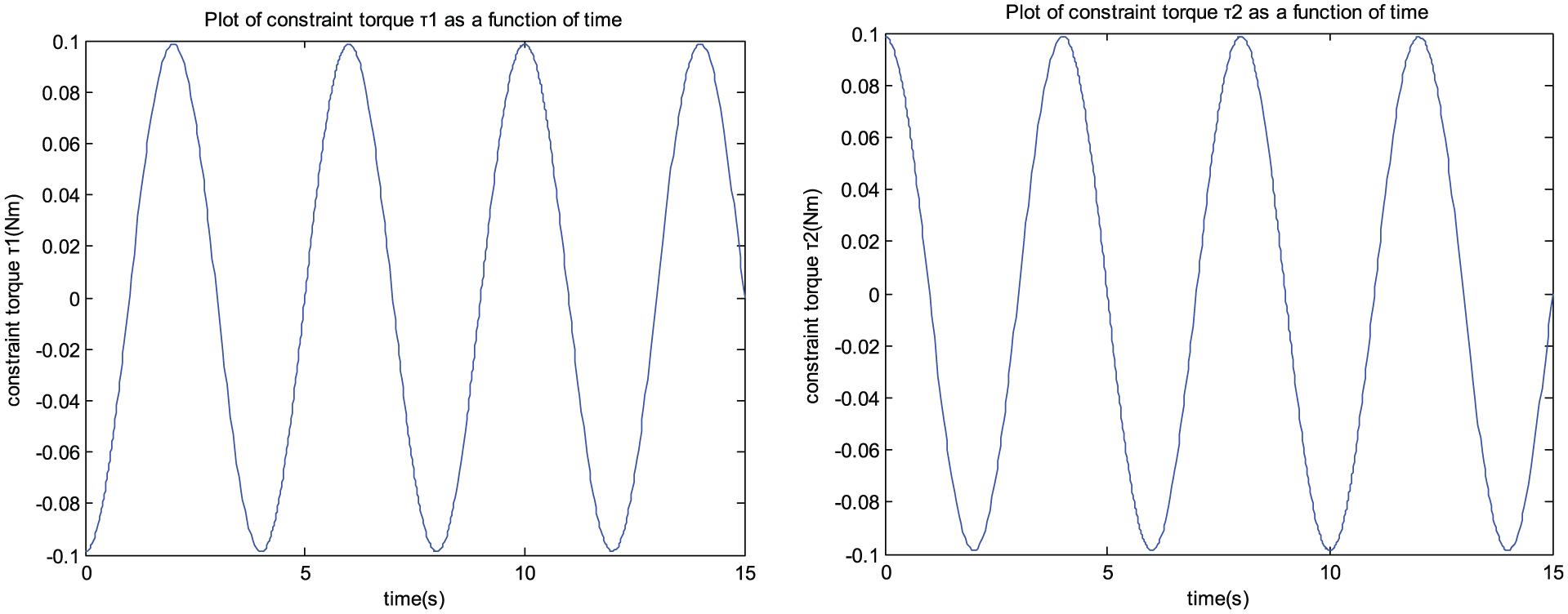
The calculated position is given in Figure 7. As shown in Figure 7, the head’s position coincides well with the desired motion (49). The calculated servo joint forces are displayed in Figure 8.

Calculated position of the snake’s head versus time (sine trajectory).

Calculated required servo joint forces versus time (sine trajectory).
The tracking errors of head’s position as functions of time are given in Figure 9. We can see clearly from Figure 9 that the tracking errors

Position error of the snake’s head versus time: (a) position error of x direction versus time and (b) position error of y direction versus time (sine trajectory).
An intuitive description of the trajectory tracking performance is shown in Figure 10. It is clear from Figure 10 that the tracking error is small enough, indicating an excellent tracking performance.
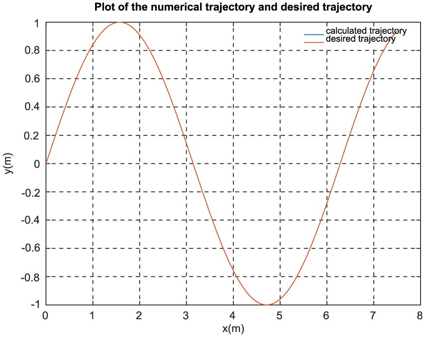
Calculated/desired trajectory of the snake’s head (sine trajectory).
Conclusion
In this article, a novel approach for the trajectory tracking control of a passive-wheel snake robot is proposed based on Udwadia–Kalaba theory. Nonlinear dynamic model of the snake is derived, and a desired trajectory is designed to illustrate this approach. The theoretical analysis and MATLAB simulation results indicate that the servo constraint control based on Udwadia–Kalaba equation fulfills the trajectory tracking task of the snake. The servo constraint torques are obtained conveniently, and the snake head movement meets the designed trajectory precisely.
The snake is a classical many-degree-of-freedom under-actuated mechanical system with characteristics of nonlinearization and nonholonomic constraints and that its dynamic modeling and controller design is relatively difficult using common methods. This article provides a novel perspective for the modeling and control problem of the passive-snake robot. The main contributions of this article are as follows:
The modeling process is easy to handle, very useful in dynamic modeling of a snake, and the constraints can be easily modeled in the analytical Udwadia–Kalaba fundamental equation. The constraints can be holonomic as well as nonholonomic, and what we need to do is just differentiate the constraints (3) and (4) with respect to time t once or twice and transform it into the form of equation (5), more efficient compared to common methods. The desired trajectories are treated as constraints named trajectory tracking constraints in Udwadia–Kalaba theory, which can be written in the form of equation (5). The passive wheels’ nonholonomic constraints can also be easily modeled by differentiating the constraints once with respect to time t.
Although many researchers proposed modified control methods to improve the tracking performances of the passive-wheel snake, these methods either make linearization or approximation of the nonlinear system or use extra variables such as Lagrangian multiplier or impose a priori structure on the nature of the controller, which is complicated and inefficient, and the tracking performance is always not optimistic. Using Udwadia–Kalaba theory, analytical equation of motion is acquired, it is exact, and no approximation of the equation of motion or modification of the controller is needed, producing an excellent control performance.
Footnotes
Academic Editor: Mario L Ferrari
Declaration of conflicting interests
The author(s) declared no potential conflicts of interest with respect to the research, authorship, and/or publication of this article.
Funding
The author(s) received no financial support for the research, authorship, and/or publication of this article.