Sage Journals: Discover world-class research

Abstract

The hybrid atomistic-continuum coupling method based on domain decomposition serves as an important tool for the micro-fluid simulation. There exists a certain degree of parallelism load imbalance when directly using the USHER algorithm in the domain decomposition–based hybrid atomistic-continuum coupling method. In this article, we propose a grid-based parallel algorithm for particle insertion, named WI-USHER, to improve the efficiency of the particle insertion operation when restricting the size of the region to be inserted or with higher number density. The WI-USHER algorithm slices the region to be inserted into finer grids with proper spacing scale, marks parts of finer grids in black according to three exclusive rules, that is, Single Particle Occupation (SPO), Single Particle Coverage (SPC), and Multi-Particles Coverage (MPC), and finds the target insertion point in the remained white grids. We use two test cases to show the superiority of our WI-USHER algorithm over the USHER algorithm. The WI-USHER algorithm performs lower averaged force evaluation times, which decreases from $O (10^{4})$ to $O (10^{3})$ compared to the USHER algorithm when the number density of slightly high to high value. The percentage of the total parallel simulation time processed by the particle insertion operation decreases from 23.5% to 3% compared to the USHER algorithm.

Keywords

Hybrid atomistic-continuum method three exclusive rules WI-USHER finer grid load imbalance

Introduction

In recent years, with the rapid development of nano-technology, micro/nano-scale devices such as micro-electromechanical system (MEMS) devices and lab-on-a-chip devices have been widely used. The fluid flows in these devices involve a broad range of scales from the atomistic scale to the macroscopic scale.^1–3 Simulation of such devices, that is, MEMS and lab-on-a-chip, cannot be carried out relying solely on the continuum models, in particular, the most commonly used Navier–Stokes (NS) equations. The NS equations become generally invalid when the continuum or thermal equilibrium condition breaks down. Molecular techniques, such as molecular dynamics (MD), can describe materials from the nanoscopic perspective and model the physics accurately at these scales. However, due to the computationally expensiveness, they cannot be directly used as a design tool for engineering nano- and micro-scale fluidic systems. In order to investigate these phenomena, researchers usually use the multi-scale modeling methods. The advantages of the multi-scale modeling lie in the ability of revealing properties of multi-scale systems by capturing phenomena that appear a wide range of time and length scales which beyond any single solver and method.⁴ Especially, the hybrid atomistic-continuum method (HAC)⁵ based on geometric coupling has seen rapid development since it allows on-the-fly information exchange and interaction between multiple simulation regions. The HAC method based on the geometric coupling obtains both simulation accuracy and efficiency, which calculating the majority of the domain by fast continuum solvers (computational fluid dynamics (CFD)) which are several orders of magnitude faster than molecular simulation methods (MD) can speed up the computation tremendously.

The HAC method splits the simulation domain into the continuum region, the atomistic region, and the overlap region, which exchanges the simulation data between the previous two regions to keep the physical properties consistently, that is, density, velocity, temperature, and so on. The top of the overlap region is the junction of the atomistic region and the continuum region, which can be regarded as an open MD simulation boundary. The MD simulation of the open boundary needs to consider the mass, momentum, and energy transfer, which is also an important feature of the simulation of non-equilibrium problem using the coupling method. One of the biggest challenges faced is the problem of the efficient insertion of particles on the open boundary in the dense liquids.⁶ To deal with the on-the-fly exchanging matter with surroundings, researchers focus on finding the efficient insertion of particles in dense liquids.

In previous studies, the most famous particle insertion algorithm is the USHER algorithm^6,7 for single particle insertion in dense fluid. For single particle insertion, the USHER algorithm randomly chooses the initial position, performs an iterative search method, which is similar to the Newton–Raphson method to find the target point based on the local potential landscape. It is default a sequential algorithm. After this, the improved algorithm of particle insertion algorithm is very little until year 2014. The FADE mass-stating technique⁸ uses a weighting function to insert and delete particles with a relaxation time. It inserts particles when the weight of the particle becomes 1 and deletes particles when becomes 0. The FADE mass-stating suits for the single particle, molecular, and even polymer. The performance of the FADE mass-stating technique matches the USHER algorithm and it is a parallel algorithm.

Nevertheless, there are still some issues to be investigated when directly using the USHER algorithm in the simulation. First, in the actual test, when the number density of the region to be inserted is larger than 0.8, the performance of the USHER algorithm decreases fast. The algorithm may not find the target position matching the threshold when reaching the maximum iteration times. Second, when we apply the USHER algorithm into the HAC coupling framework⁹ because of the limitation of the insertion volume, the USHER algorithm appeals the same deficiency performance as the high value of number density. Third, there will be multiple regions to be inserted particles into in the parallel HAC simulation. After each particle insertion operation, the whole simulation system has to update the total particle number to each process. Different insertion performance of each process results in long-time synchronization barrier. The imbalance of parallel insertion operation leads decreasing in parallel simulation performance. Therefore, there is an urgent need to improve the performance of the particle insertion operation.

In this article, focusing on the computational efficiency of the particle insertion operation in the hybrid coupling simulation, we propose a grid-based parallel particle insertion algorithm modified from the famous insertion algorithm USHER.⁶ Specifically, the main contributions of this article are summarized as follows:

We analyze the deficiency of the original USHER algorithm, formalize the problem of particle insertion, and put forward the solution to the deficiency of the particle insertion.

We propose the WI-USHER parallel algorithm for the HAC method. The algorithm slices the region to be inserted into finer grids, marks some grids black according to three exclusive rules, that is, SPO, SPC, and MPC, and uses the steepest descent method to find the target position in the remained white grids.

We implement the WI-USHER algorithm in our HAC coupling framework based on OpenFOAM¹⁰ and LAMMPS.¹¹ Comparing with the USHER algorithm under the simulation of the number density from slightly high value to high value, the averaged force evaluation times of the WI-USHER algorithm decreases an order of magnitude from $O (10^{4})$ to $O (10^{3})$ and the percentage of the total simulation time processed by the particle insertion operation reduces from 23.5% to 3%.

The remainder of the article is organized as follows: section “Preliminary” reviews the HAC simulation methodology and the particle insertion algorithm. Section “Basic idea of White Initial USHER parallel algorithm” uses two cases to present the deficiency of the original USHER algorithm, formalizes the particle insertion problem, and proposes the basic idea of our WI-USHER algorithm. Section “Algorithm and implementation” presents the key exclusive rules of the WI-USHER parallel algorithm and gives the design and implementation of the algorithm based on OpenFOAM and LAMMPS. Section “Experiments” evaluates the efficiency of our WI-USHER compared with the USHER algorithm using two benchmark cases. Finally, Section “Conclusions” concludes the article.

Preliminary

In this section, we review the HAC coupling method and framework based on domain decomposition and the existing algorithm of particle insertion operation.

Hybrid coupling computational framework

With the rapid development of high-performance computing (HPC), the simulation ability of classical MD is extended but still cannot fulfill very large-scale particle simulation application. HAC method limits the use of MD simulation to regions where the atomistic scales needed to be resolved, while using a continuum-based solver for the remainder of the domain, which obtain both simulation accuracy and efficiency.

The first hybrid method combining MD with the continuum method for dense fluid was proposed by O’Connell and Thompson.⁵ For the two-dimensional (2D) Couette flow, the domain was split into an atomistic region and a continuum region, using an overlap region to alleviate dramatic density oscillation and couple the results of these two regions. The outer boundary of the continuum region which resides in the atomistic region is called hybrid solution interface (HSI). Later, HAC models emerged differing in forms of coupling strategies, boundary conditions extraction, and non-periodic boundary force models.^4,12,13 We name the atomistic region and the overlap region unified as the particle region for that MD simulation performing on both of these two regions. We use the abbreviation “A” for the “atomistic” and “C” for “continuum.” Generally, the overlap region contains a control region (control region), a buffer region (buffer region), an atomistic-coupled-to-continuum-region (A → C region), and a continuum-coupled-to-atomistic region (C → A region). In the control region, there is a reflecting wall boundary condition to prevent particles leaving the atomistic region freely and the outer boundary is the MD–continuum interface. The schematic diagram of the domain decomposition–based HAC method is depicted in Figure 1.

Figure 1.

Domain decomposition of benchmark case, channel flow past the rough wall and detailed of the overlap region. “A” is the abbreviation for “atomistic,” while “C” is for “continuum.” Yellow dots represent fluid particles and black dots for solid wall particles.

In order to facilitate data exchanging between the continuum solver and the atomistic solver, the overlap region is sliced into bins to match the cells in the continuum region as shown in Figure 2. There are four layers of bins which are corresponding to the control region, C → A region, buffer region, and A → C region. In the continuum region, we use the incompressible NS equation for modeling the system. The NS equation and the continuity equation are given by

\nabla \cdot u = 0

(1)

\frac{\partial u}{\partial t} + \nabla \cdot (uu) = - \frac{1}{ρ} \nabla P + ν \nabla^{2} u

(2)

where $u$ is the bulk flow velocity, P is the pressure, and $ν$ is the kinematic viscosity. The equations above are solved numerically using the finite volume method.

Figure 2.

Diagram of particle insertion occurring on the atomistic-continuum interface. $u_{i}^{α}$ is the macroscopic velocity in the y-direction here. $A_{i}$ is the surface area perpendicular to $u_{i}^{α}$ .

In the particle simulation, we use the truncated and shifted Lennard–Jones (LJ) potential to model the interactions between fluid particles and wall particles. The potential is given by

ϕ (r) = {\begin{matrix} 4 ϵ [{(\frac{σ}{r})}^{12} - {(\frac{σ}{r})}^{6} + {(\frac{σ}{r_{c}})}^{12} + {(\frac{σ}{r_{c}})}^{6}], r \leq r_{c} \\ 0, r > r_{c} \end{matrix}

(3)

where $r_{ij}$ is the distance between atom i and j, $r_{c}$ is the cutoff radius, and $ϵ$ and $σ$ are the characteristic molecular energy and the molecular length scale, respectively.

The parallel hybrid coupling framework based on the domain decomposition consists of the continuum solver (CFD solver), the atomistic solver (MD solver), and relatively coupling operations. The parallelization of the continuum part is based on mesh decomposition, while the atomistic part is on simulation domain decomposition to allocate sub-mesh and sub-domain on each process. Reasonable parallel coupling operations play an important role on efficient coupling simulation. There are also different multi-scale coupling methods, that is, finite volume method and lattice Boltzmann method,¹⁴ finite volume method, and Brownian configuration method.¹⁵ The existing coupling method frameworks include MaMiCo.¹⁶

Particle insertion algorithm

In order to exchange mass flux with the open boundary, the USHER algorithm^6,7 uses a Newton–Raphson liked method to iteratively find the target position according to the local potential landscape. Many existing research deals with the mass flux using this method.^17,18 The target position of a new inserted particle is where the potential is equal to the average potential of the whole region to be inserted or within a pre-set threshold of the average potential. In practice, the pre-set threshold is usually a small value, that is, 0.001. One attempt of insertion involves first keeping all the other particles in the region frozen in space and time. A new trial particle is then inserted randomly in the region and is shifted away from the overlapping core of resident particles in an iterative manner, guided by the strength and slope of the static potential energy landscape. Once the target position is found, the new particle is assigned with velocity drawn from the Maxwell-Damon distribution according to the temperature of the whole region.

In the HAC method based on the domain decomposition, the MD–continuum interface needs the particle insertion algorithm to exchange mass flux between the continuum region and the atomistic region. When applying the USHER algorithm into the coupling method, a control region should be introduced to complete this operation as depicted in Figure 1. Furthermore, in order to complete data exchanging, the overlap region has to be sliced into bins to match the mesh cells of the continuum region as shown in Figure 2.

In previous studies, for the mass exchange of the open boundary, the conventional method is to convert the mass flux into the number of particles using a converted equation and utilize the insertion and deletion particles of the MD region to characterize the exchange of mass flux. In one CFD time-step, the number of particle to be inserted or deleted is calculated using equation (4)

n = (\frac{A_{i} ρ u_{i}^{α} Δ t_{CFD}}{m})

(4)

where $A_{i} = (Δ x \times Δ z) \cdot n$ is the surface area perpendicular to the direction y, $n$ is the surface vector, pointing to the atomistic region. $u_{i}^{α}$ is the continuum velocity in the inserted bin, $ρ$ is the liquid density, and m is the particle mass. If n is positive, it means inserting particles into the atomistic region, otherwise delete particles.

When continuously inserting particles into the region, the USHER algorithm needs to recalculate the region energy every insertion, because of that after each new insertion, the local potential landscape changes with every insertion. Borg et al.⁸ point out that the main disadvantages of the USHER algorithm are that it requires the correct selection and optimization of the input parameters to minimize computational cost and maximize insertion rate, but they do not further investigate these disadvantages.

In this article, we modify the USHER algorithm to apply it into our HAC coupling framework,⁹ analyze the deficiency of the USHER algorithm, and make the particle insertion operation more efficiency for the coupling simulation.

Basic idea of White Initial USHER parallel algorithm

In this section, we present the basic idea of our WI-USHER parallel algorithm. Subsection “Deficiency of the USHER algorithm” uses two cases to reveal the deficiency of the original USHER algorithm. Section “Formulation of particle insertion algorithm” formalizes the particle insertion problem. Section “WI-USHER parallel algorithm” gives the basic idea of the exclusive method.

Deficiency of the USHER algorithm

The authors of the USHER algorithm choose the initial start position totally randomly. In order to test the insertion efficiency of the USHER algorithm, Delgado-Buscalioni and Coveney⁶ choose constantly inserting into a periodic box. In this test case, the volume of the simulation domain keeps unchanged, there is no external thermo bath, and the motion of Argon particles is governed by Newtonian equation. We initialize the same periodic box 10 times with different random numbers. The pre-set threshold is set as 0.001 and the maximum iteration times of iteratively searching are set as 5 × 10⁴. The initial number density is 0.8 and we insert new particles into the periodic box with a constant insertion rate until the number density reaches 1.0. The algorithm will reach the maximum iteration times when it cannot find the position with potential that satisfies the threshold. The force evaluation times needed by each insertion is categorized in Table 1.

Table 1.

Distribution of force evaluation times with maximum iteration times 5 × 10⁴.

Evaluation times	Frequency number	Probability (%)
>5 × 10⁴	73	36.5
500∼5 × 10⁴	64	32
100∼500	43	21.5
<100	20	10

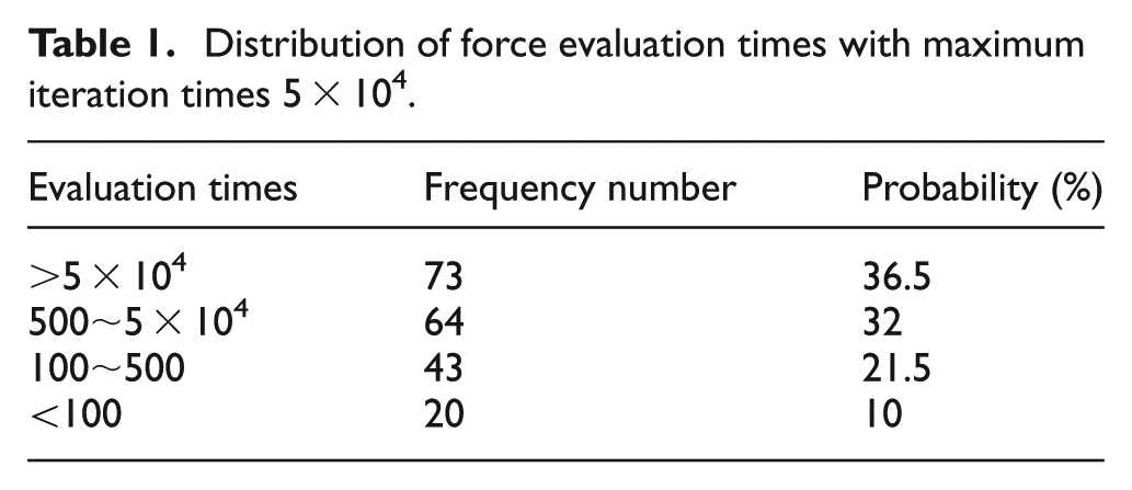
From Table 1, we find that the force evaluation times that reaches the maximum iteration times is with the probability of 36.5% as the number density of the inserted region increases. The force evaluation times that reaches the maximum number means the USHER algorithm does not find the target position meeting the threshold but find sub-optimal position. Moreover, in order to exclude the effect of the maximum iteration times, we choose another pre-set maximum iteration times 1 × 10⁶. The test results are shown in Table 2.

Table 2.

Distribution of force evaluation times with maximum iteration times 1 × 10⁶.

Evaluation times	Frequency number	Probability (%)
>1 × 10⁶	66	33
500∼1 × 10⁶	69	34.5
100∼500	47	23.5
<100	18	9

Due to a different maximum iteration times, when one insertion attempt reaches the maximum, there will be different sub-optimal positions among different maximum times, and later insertions will be slightly different. We find that even increasing the maximum iteration times, in some insertion attempts, it cannot find the optimal position yet.

Especially, the deficiency of the USHER algorithm becomes worse when applied into the HAC method. During the parallel coupling simulation, there would be multi-regions to be inserted as the same insertion operation. After each coupling operation, all the processes have to be synchronized because of the variation of total particle number. If the USHER algorithm in one of the inserted regions reaches the maximum iteration times, the other processes have to wait until this process finishing iteration. During the whole coupling simulation, insertions probably happen on different process. Parallel insertion imbalance seriously impacts the parallel performance. The schematic of parallel insertion and synchronization is depicted in Figure 3 with four processes (Q0, Q1, Q2, and Q3).

Figure 3.

Schematic diagram of parallel particle insertion and barrier with the degree of parallelism 4. Taking t to $t + 3 Δ t$ as an example.

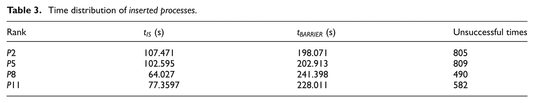
We take a HAC case with 12 degree of parallelism as an example to depict the parallel insertion imbalance. The continuum region is decomposed into 4 × 3 sub-meshes and the particle region, that is, the atomistic region and the overlap region, is decomposed into 4 × 3 sub-domains. The parallel partition of the particle region is shown in Figure 4, which only process P2, P5, P8, and P11 would perform the particle insertion operation, named as inserted processes.

Figure 4.

Schematic diagram of processes distribution in the atomistic region (gray) and the overlap region (light green) with the degree of parallelism 12.

The whole simulation time is 8 ns. The time step of MD is 0.005τ and the time step of CFD is 100 times the MD time step. The total time steps of MD is 8 × 10⁵ and CFD is 8 × 10³. The total computation time includes three parts: the CFD computation time $t_{CFD}$ , the MD computation time $t_{MD}$ , and the coupling operation time $t_{CO}$ . We take more consideration on the particle insertion time $t_{PI}$ which is a part of $t_{CO}$ . For the parallel particle insertion, the particle insertion time $t_{PI}$ of the USHER algorithm is further divided into iterative search time $t_{IS}$ and barrier time $t_{BARRIER}$ . The distribution of the computation time of four inserted processes is shown in Table 3 and the distribution of the whole computation time is listed in Table 4.

Table 3.

Time distribution of inserted processes.

Rank	$t_{IS}$ (s)	$t_{BARRIER}$ (s)	Unsuccessful times
P2	107.471	198.071	805
P5	102.595	202.913	809
P8	64.027	241.398	490
P11	77.3597	228.011	582

Table 4.

Time distribution of each procedure.

	t_CFD (s) (%)	t_MD (s) (%)	t_CO (s) (%)	t_PI (s) (%)
Time	47.03 (3.598)	862.49 (65.99)	397.46 (30.5)	307.08 (23.95)

From Tables 3 and 4, we find that the particle insertion operation time processes the main part of the coupling operation time due to unsuccessful insertions. Because only part of processes involved in the particle insertion, the long-time insertion and barrier of these processes destroy the parallel performance of the hybrid simulation.

We have discussed the deficiency of the USHER algorithm using two bench cases. The USHER algorithm that totally chooses the initial position randomly does not perform perfectly, but limits the parallel efficiency of the coupling simulation. Therefore, there is an urgent need to improve particle insertion performance.

Formulation of particle insertion algorithm

The present particle insertion algorithms are mostly based on the potential distribution in the region to be inserted and use the evolution of the local potential to iteratively find the appropriate position. In the USHER algorithm, the potential energy of the newly inserted particle is approximately equal to that of the excess potential energy per particle u the system, that is, $u = U / N$ , where U is the potential of the region to be inserted and N is the number of particles in the region. The insertion of such a new particle position has no damage to the statistical features of the original system.

After continuously inserting into the periodic box, we find that the final target position is a position that the distances between the newly particle and surrounding particles are proper. This proper means there is an empty sphere that consists only the newly introduced particle. Under the hard sphere assumption,¹⁹ the particle is presented with the center of the sphere $(x, y, z)$ and a reasonable radius r. Therefore, two particles cannot get two close to each other. According to the LJ potential, when the distance between two particle is smaller than $1 σ$ , the potential increases dramatically. In the normal state, the distance between each particle pair is reasonable and the newly introduced particle should have the reasonable distance with surrounding particles.

Therefore, if there is a sufficient large empty sphere in the region to be inserted, there will a target position in such an empty sphere that meets the requirement of the particle insertion algorithm that has no damage on the statistical features. We give such a lemma of the newly introduced particle.

Lemma 1

If there is sufficient large empty sphere in the region to be inserted, there must have such a position in the empty sphere that meets the potential requirement. On the contrary, if there is no such an empty sphere, under such configuration of the region to be inserted, there will have no target position.

In order to find a target position in a point source field, we can reference to the solution of finding the Largest Empty Sphere (LES) in three-dimensional (3D) (Largest Empty Circle (LEC) in 2D). The problem of finding the LES can be solved using Voronoi diagram.²⁰

LES problem

Given a set $S_{p}$ of N points $s^{i}, i = 1, \dots, N$ , in a bounded space S, find the point p in S from which the distance to the nearest point among the set is the longest, that is

\max_{p \in S} \min_{i} d (p, s^{i})

(5)

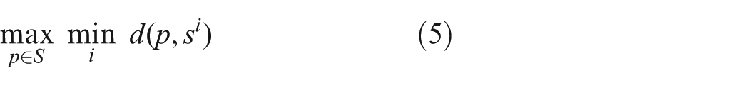
where $d (p, q)$ is the distance between two points p and q.

For 2D LEC problem, the time and space complexity of using Voronoi diagram are $O (N \log N)$ and $O (N)$ . While in 3D, the complexity goes up to $O (N^{(n + 1) / 2})$ . The modified algorithm of the LES problem is scarce.^21,22 When inserting a new particle to a point source field, we can only refer to the existing of configuration of particle positions.

WI-USHER parallel algorithm

In the previous section, we formalize the problem of particle insertion and find that we can choose the newly particle position only according to the configuration of the existing particle positions. But, in 3D, the complexity of space and time is sufficiently high. Taking a system of 800 particles as an example, the complexity of finding a empty sphere matching the threshold is $O (N^{(n + 1) / 2}) = 6.4 \times 10^{5}$ , which is quite higher than the pre-set maximum iteration times mentioned in subsection “Deficiency of the USHER algorithm.” Therefore, the forward method of finding the Empty Sphere in the source field is too costly. In the hybrid coupling simulation, the time complexity is not acceptable.

As we know, the original USHER algorithm chooses the initial position totally randomly and not refers to the configuration of particles in the system. Therefore, we combine the idea of finding the LES and some exclusive rules, which exclude some parts of the region that exist no target positions and use the local potential landscape to find the target position in the remaining parts.

It is the starting point of the WI-USHER algorithm that eliminates those spatial region existing no target points, named impossible region and uses the remained white initial region to search the target. Through profiling the configuration of existing particles, the WI-USHER algorithm combines the particle effective sphere as shown in Figure 5 and excludes the impossible region. The effective sphere represents the ability of one particle marking the inserted region. For there is difficulty of describing the effective sphere in the algorithm, we use the finer grids method that slices the region to be inserted into multi finer grids. Each particle has its own belonging grid and the effective sphere that can cover the neighbor grids. Multi-particles have the union coverage of finer grids to further exclude impossible region. The detailed definition of the effective sphere is presented in section “Algorithm.”

Figure 5.

Schematic diagram of the effective sphere for single particle. The grids that are not marked in black are the White initials for the WI-USHER algorithm.

We can find that in order to describe the configuration of the particles position information, we must introduce some data structures to maintain these information. If any inserted process reaches the maximum iteration times, it will delay the overall performance of the parallel simulation, so it is feasible to exchange the time efficiency method through spatial storage.

Algorithm and implementation

In this section, we present the detailed design of our WI-USHER algorithm and the implementation in our hybrid coupling framework. Section “Algorithm” gives the parameters involved in the algorithm and section “Data maintenance and implementation” presents the maintenance data info and the implementation in our hybrid coupling framework. We choose the liquid argon as the model fluid. The reason for selecting argon as the fluid for simulation is that the particles have well-established atomic potential interaction and it serves as a reference point for more complex fluid simulations. We choose the shifted LJ potential, whose parameters are $σ = 0.34 nm$ , $ϵ = 1.67 \times 10^{- 21} J$ , particle mass $m = 6.63 \times 10^{- 26} kg$ , and the cutoff radius $r_{c} = 2.2 σ$ .

Algorithm

The key idea of the WI-USHER algorithm is to eliminate those impossible regions and to guide the location of the target points may exist more inclined. The algorithm slices the region to be inserted into finer grids. The direction of building finer grids is to slice each particle into one grid. The exclusive rules of the WI-USHER algorithm are SPO, SPC, and MPC which are discussed in the following sections.

Single particle occupation

In this article, we take the liquid argon as the model liquid and the LJ potential as the pair interaction potential as shown in Figure 6. From the distribution of the potential, we can see that under the hard sphere approximation, each particle has its reasonable radius and particles cannot get too close to each other. We give the definition of the healthy distance when the particle pair distance is larger than $0.95 σ$ and the definition of the vicious distance when the distance is smaller than $0.95 σ$ .

Figure 6.

Lennard–Jones 12-6 potential.

The spatial selection of finer grids is properly chosen that each particle belongs to only one grid. The first exclusive rule is SPO, which means the grid that one particle belongs to would not exist the target position. The procedure of the WI-USHER algorithm is slicing the region to be inserted to finer grids as shown in Figure 7 and then marking the grids in black that have particle belongs to as shown in Figure 8.

Figure 7.

Initial finer grids for the inserted region, each finer grid occupies only one particle with proper spatial slicing.

Figure 8.

Single Particle Occupation exclusive rule, each grid that occupied by the particle should be marked in black.

Single particle coverage

Based on the assumption of the hard sphere, each particle has its effective diameter. Therefore, we use the $r_{E}$ to represent the effective coverage radius, that is, the radius of the effective sphere. This reasonable coverage depends on the physical properties of the particle. The definition of it is the largest coverage that a single particle can reach. Through the definition of the vicious distance, each grid covered in the vicious distance exist no target position.

In 3D problem, the measured distance is the largest distance between the eight corners of the grid and the particle. The procedure of the WI-USHER algorithm goes on to mark black to those grids within the coverage of a single particle, that is, the second exclusive rule SPC as shown in Figure 9.

Figure 9.

Single Particle Coverage exclusive rule, each grid within one of the effective sphere should be marked in black.

Multi-particles coverage

In the previous two sections, we exclude grids according to the SPO and the SPC. Next, we discuss the union coverage of multi-particles to mark grids black.

Due to the effective coverage of a single particle in a sphere, the overlap of one sphere and one grid is measured whether the eight corners of the grid are in the sphere or not as shown in Figure 10. If one grid is covered by multi-particles to a certain value, it will be marked in black, that is, the third exclusive rule MPC.

Figure 10.

Multi-Particles Coverage exclusive rule, each grid that covered by the multiple effective sphere to a certain value should be marked in black.

The detail of this overlapping measurement is described as follows. The proper spatial parameter of finer grids that we choose is contained only one particle in each grid and the largest distance between the center of one grid to the eight corners of the neighbor grid is larger than the effective radius $r_{E}$ . For each particle $s^{i} (x, y, z)$ with effective coverage $r_{E}$ , we could only take 26 neighbor grids (in 3D) around it into consideration. The corner of each grid is $c^{i} (i = 1, \dots, 8)$ . The percentage of coverage is defined as follows

Coverage percentage = \frac{\sum vol (\max_{i} r (c^{i}, s^{i}) < r_{E})}{Vol of grid}

(6)

There are three situations that one gird covered by one particle effective coverage, we deal with them separately:

Totally covered. If the largest distance between the eight corners and the particle is smaller than $r_{E}$ , the grid is totally covered.

Totally uncovered. If the smallest distance between the eight corners and the particle is larger than $r_{E}$ , the grid is totally uncovered.

Partial covered. The largest distance between the eight corners of the grid and the particle is larger than $r_{E}$ while the smallest distance is smaller than $r_{E}$ . There are lots of previous study to discuss the overlap between the sphere and the grid.²³ Taking the efficiency of the calculating algorithm, we choose another way that if it is partial covered, we cut the grid into eight sub-grids and further consider the overlap of the sphere and eight sub-grids. When the volume of the sub-grid is only 5% of the original one, we will stop sub-dividing the grid. Especially, the coverage part of the grid by multi-particles is tallied only once when some parts of the grid are covered by two or more particles simultaneously.

The pseudo-code of the particle coverage is shown in Algorithm 1.

Algorithm 1. Algorithm for the particle coverage calculation.
Require: particle $a_{i} (x_{i}, y_{i}, z_{i})$ , grid_extent, grid_cover_tag, $r_{E}$
Ensure: all neighbor grids have been considered
1: calculate grid volume vol and eight corner points $c_{i}$ of the grid
2: if $\max dis (c_{i}, a_{i}) < r_{E}$ then
3: the grid is all in the coverage, return the grid vol, fill in grid_cover_tag
4: end if
5: if $\min dis (c_{i}, a_{i}) > r_{E}$ then
6: the grid is all out of the coverage, return 0
7: end if
8: if $vol < SMALL$ then
9: the grid vol is very small, return 0
10: end if
11: split the grid into 8 sub-grids, reconsider the above operations

After these three rounds of exclusion, the region that may exist target positions is narrowed to nearly 30% or less of the original region to be inserted. The WI-USHER algorithm will find the target position in the remained white initial grids. In the remained white initial grids, the WI-USHER algorithm will tally each of these grids, by finding a position in some grids with the potential equals to the average potential of the inserted region. The initial insertion point in each grid is randomly chosen and updated by Newton–Raphson method that only goes down the direction of the landscape of the energy potential in the inserted region. When the energy potential goes up, the WI-USHER algorithm will pass this grid and go on tally the other grids until finding the target position with the desired energy as the same method in Delgado-Buscalioni and Coveney.⁶

Data maintenance and implementation

When the insertion happens during the simulation, particles in the region to be inserted are varied each time, so the relationship between particles and finer grids is needed to recalculate each insertion. The WI_USHER algorithm needs certain data structures to maintain the relationship. In our hybrid coupling framework, we implement the parallel version of the WI-USHER algorithm to meet the simulation requirement.

Definition of data maintenance

The WI-USHER algorithm needs to define the spatial info of finer grids and the neighbor relationship. In each insertion attempt, we should profile the following messages:

The relationship between particles and the region to be inserted: in the region to be inserted or within the cutoff of the region to be inserted;

The relationship between particles and finer grids: particle numbers and particle positions in each grids;

The marking information of finer grids.

After profiling the above messages, the WI-USHER algorithm uses these configuration info to exclude region to be inserted and improve the performance of the particle insertion operation.

Implementation and parallelized design

In this article, we implement our WI-USHER algorithm in the HAC software framework based on OpenFOAM and LAMMPS. OpenFOAM serves as the main solver and LAMMPS is used as a dynamic library to be called from OpenFOAM. The solver is an incompressible, single phase, Newtonian solver to accomplish the coupling simulation. The WI-USHER algorithm is implemented as a fix style command in LAMMPS. As there are multi-regions to be inserted during the coupling simulation, we need to deal with the newly created particles overlapping between neighbor processes as shown in Figure 11.

Figure 11.

Diagram of neighbor process overlapping checking, only checking with neighbor who also has particle insertion operation.

In the coupling simulation, the degree of parallelism is $N_{p}$ . The mesh of the continuum region is decomposed into $N_{p}$ sub-mesh and the domain of the atomistic region is also into $N_{p}$ sub-domain. As only some processes are inserted processes, they have to check the newly created particles overlapping with each other using Algorithm 2 and they have to check the local created particle overlapping.

Algorithm 2. Algorithm for neighbor processes overlapping checking.
Require: rank i for $P_{i}$ , new created position $(x_{i}, y_{i}, z_{i})$ ,processes neighbor info
Ensure: all inserted $P_{i}$ find new created position
1: for $di m_{i} \in [1, 3]$ do
2: if left neighbor is inserted processthen
3: send local new created positions to left neighbor
4: end if
5: if right neighbor is inserted processthen
6: receive neighbor new created positions from right neighbor
7: end if
8: check whether has overlapped positions
9: if position overlapped then
10: remove local new created position
11: end if
12: end for

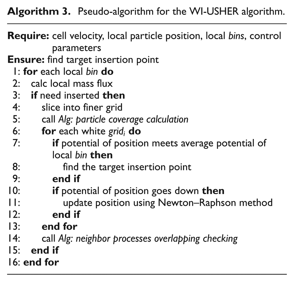
The detailed procedure of the WI-USHER algorithm in depicted in Algorithm 3.

Algorithm 3. Pseudo-algorithm for the WI-USHER algorithm.
Require: cell velocity, local particle position, local bins, control parameters
Ensure: find target insertion point
1: for each local bindo
2: calc local mass flux
3: if need inserted then
4: slice into finer grid
5: call Alg: particle coverage calculation
6: for each white $gri d_{i}$ do
7: if potential of position meets average potential of local binthen
8: find the target insertion point
9: end if
10: if potential of position goes down then
11: update position using Newton–Raphson method
12: end if
13: end for
14: call Alg: neighbor processes overlapping checking
15: end if
16: end for

Experiments

We demonstrate the superiority of the WI-USHER algorithm over the original USHER algorithm using two test cases and also list the worst case of our WI-USHER algorithm. Section “Platforms” introduces the platform we used, section “Periodic box” shows the analysis and results of the first case with periodic boundary condition, section “Channel flow past the rough wall” gives the analysis and results of the second case with rough boundary condition, and section “Worst case” presents the worst case of our modified algorithm.

Platforms

In the experiments, we use a HPC cluster situated in the State Key Laboratory of High Performance Computing.²⁴ This computing platform consists of hundreds of computing nodes and each node contains 12 Intel Xeon 2.1 GHz E5-2620 CPU cores and a total memory of 16 GB. We implement our HAC coupling framework using OpenFOAM, which is an excellent CFD open-source software with C++ object-oriented class libraries, and LAMMPS, which is a classical MD simulation code.

Periodic box

The first test case is a periodic box with liquid argon as mentioned in Delgado-Buscalioni and Coveney,⁶ whose length is $L = 10 σ$ . We compare the performance of our WI-USHER algorithm and the USHER algorithm when the number density is slightly high and high in sequential manner.

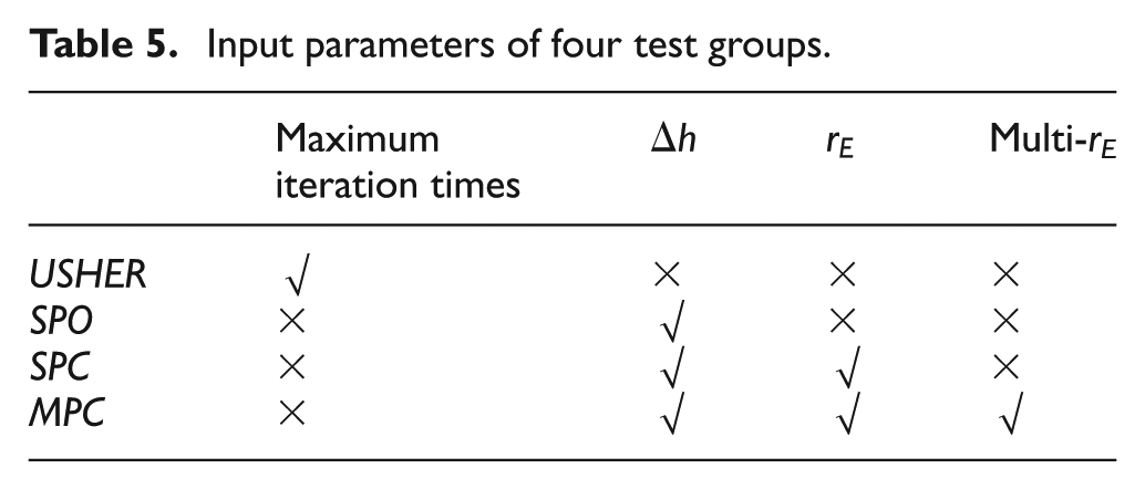
The test case is with no external thermostat to prevent the temperature of the system increasing dramatically due to improper insertion. The insertion rate is kept at a small rate, so the system can relax to equilibrium after one insertion. Under the assumption of the hard sphere, the insertion rate should be smaller than the particle collision time, which is $τ_{c} = 0.14 ρ^{- 1} T^{- 1 / 2} (σ^{2} m / ε)^{1 / 2}$ .²⁵ In order to match the coupling operation in the next case, we choose the insertion rate as inserting every 100 MD time steps. The initial number density is chosen a slightly high value, which is $ρ = 0.8$ . We keep inserting in the periodic box until $ρ = 1.0$ with 200 insertion times, that is, 2 × 10⁴ MD time steps with $t_{MD} = 0.005 τ$ . The evaluation error of particle insertion for both algorithms is set as 0.001. The pre-set maximum iteration times is set as 5 × 10⁴.

The input parameters of the WI-USHER algorithm are as follows: the effective coverage radius $r_{E}$ , finer grids spatial scale $Δ h$ . The multi-particles coverage can only be used as a supplement to the effective coverage radius $r_{E}$ . The input parameter of the USHER algorithm is the maximum iteration times. The reason for why the WI-USHER algorithm does not set the maximum iteration times is that the algorithm will search all the remained white grids without limitation. In order to meet the ensemble requirement, we run the same test 10 times with different initial random seed and present the average results of each test. We design the following four test groups to compare these two algorithms and list detailed input parameters in Table 5:

USHER: no finer grids, only set the maximum iteration times;

SPO: consider SPO of the grid, vary the grid spatial scale $Δ h$ ;

SPC: consider single particle effective coverage of the grid, vary the grid spatial scale $Δ h$ ;

MPC: consider the multi-particles effective coverage of the grid, vary the grid spatial scale $Δ h$ .

Table 5.

Input parameters of four test groups.

	Maximum iteration times	$Δ h$	$r_{E}$	Multi-r_E
USHER	√	×	×	×
SPO	×	√	×	×
SPC	×	√	√	×
MPC	×	√	√	√

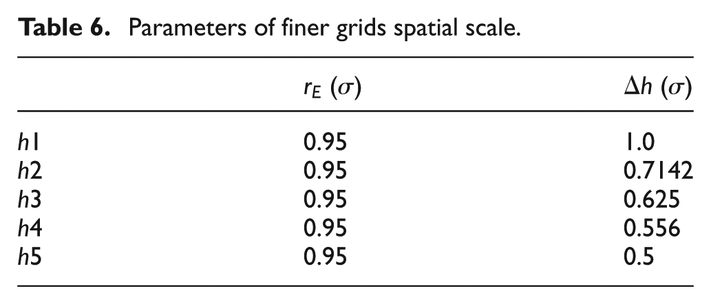
Especially, we also set five kinds of grid spatial scale for the last three test groups (SPO/SPC/MPC) to find the effect of grid spatial scale on the particle insertion operation. The effective coverage radius $r_{E}$ is set equal to the healthy distance of $0.95 σ$ . The detailed spatial parameters are listed in Table 6.

Table 6.

Parameters of finer grids spatial scale.

	$r_{E}$ ( $σ$ )	$Δ h$ ( $σ$ )
h1	0.95	1.0
h2	0.95	0.7142
h3	0.95	0.625
h4	0.95	0.556
h5	0.95	0.5

As both algorithms use the iteration searching, the final finding position of 200 times insertion may be different between the WI-USHER algorithm and the USHER algorithm. The results of the first test case are demonstrated in two parts: first, we show the validity of our WI-USHER algorithm that using exclusive rules do not damage the correctness. Physical properties such as system temperature T, system pressure P, total energy per particle and excess energy per particle $u = U / N$ varies with number density $ρ$ are evaluated. We choose the h2 spatial scale to present the results, and the results (Figures 12 –15) show the validity of our WI-USHER algorithm compared with those in Delgado-Buscalioni and Coveney.⁶

Figure 12.

Temperature for density from 0.8 to 1.0 of the periodic box case.

Figure 13.

Pressure for density from 0.8 to 1.0 of the periodic box case.

Figure 14.

Total energy per particle for density from 0.8 to 1.0 of the periodic box case.

Figure 15.

Excess energy per particle for density from 0.8 to 1.0 of the periodic box case.

Second, we compare the efficiency of these two algorithms using the average force evaluation times as shown in Figure 16, average evaluation error as shown in Figure 17 within 200 times insertion. In each insertion attempt, the kernel part is the evaluation of force that imposed by other particles. Therefore, evaluating the force times depicts the efficiency of the algorithm.⁶ At the same time, we also show the evaluation error between the target potential and the finding potential under different input parameters. These two results use the result of the USHER algorithm as the base line. Under different finer grid spatial scales, more finer the grids brings more storage consuming, on the other side, more sparer the girds, the SPC can only cover the local grid and lose the ability of covering neighbor grids. We also show the detailed insertion time info of these two algorithms, that is, the WI-USHER algorithm consists of iteratively searching $t_{IS}$ and data maintenance time $t_{DM}$ , while the USHER algorithm consists of only iteratively searching time $t_{IS}$ (Figure 18).

Figure 16.

Average force evaluation times of 200 times insertion for the WI-USHER algorithm with three exclusive rules, SPO, SPC, and MPC, and the result of the USHER algorithm is as the base line.

Figure 17.

Average evaluation error of 200 times insertion for the WI-USHER algorithm with three exclusive rules, SPO, SPC, and MPC, and the result of the USHER algorithm is as the base line.

Figure 18.

Detailed insertion time info, total simulation time, and data maintenance time of the WI-USHER algorithm, and the result of the USHER algorithm is as the base line.

From the above results, we find that the average force evaluation times and insertion time of the WI-USHER algorithm almost perform better than the USHER algorithm. The SPO test group performs a little worse for exclusion few grids than the SPC group and the MPC group, even than the USHER. The SPC group and the MPC group exclude more grids and clearly direct to the final target region. The insertion time-consuming by the WI-USHER algorithm is almost less than the USHER algorithm; furthermore, the MPC group brings in more data maintenance time but excludes more grids. Under the five finer grids spatial scale, the h3 group performs the best with three exclusive rules.

Through these four test groups, we draw the following empirically conclusion: according to the definition of healthy distance, in 3D simulation, the body diagonal of finer girds is chosen as about $1 σ$ , while in 2D, the face diagonal of about $1 σ$ . This makes sure that each grid contains at most one particle. When taking the MPC into consideration, it uses the recursively method to tally the coverage percentage of one grid, excludes more grids, but brings in storage and time-consuming. Therefore, the performance of MPC sometimes is worse than the SPC.

Channel flow past the rough wall

The second test case is the channel flow past the rough wall^17,26 as shown in Figure 19. We use this test case to compare the parallel performance of these two algorithms when existing mass flux across the MD–continuum interface. The simulation domain is $x \times y = 52.1 \times 52.1 σ^{2}$ , while the z-direction of the MD domain is $5.21 σ$ . The moving and the still wall are no slip boundary condition. The height of the CFD domain is $36.47 σ$ , consists of 12 × 7 cells and the height of the MD domain is $31.26 σ$ , consists of 10 × 6 bins. The rough bottom wall consists of two layers of face-centered cubic (FCC) (111) solid particles and the height of it is about $5 σ$ . The velocity of the top wall is $U_{w} = 1.0 σ / τ$ . The simulation time is 8 ns and the time-step of MD is $0.005 τ$ . The total MD time steps is 8 × 10⁵ and CFD is 8 × 10³. We run the simulation for 10 times with different random seed and average these 10 times for results.¹⁷ The particle insertion time $t_{PI}$ of our WI-USHER algorithm is divided into iterative search time $t_{IS}$ , data maintenance time $t_{DM}$ , and barrier time $t_{BARRIER}$ .

Figure 19.

Diagram of channel flow past the rough wall.

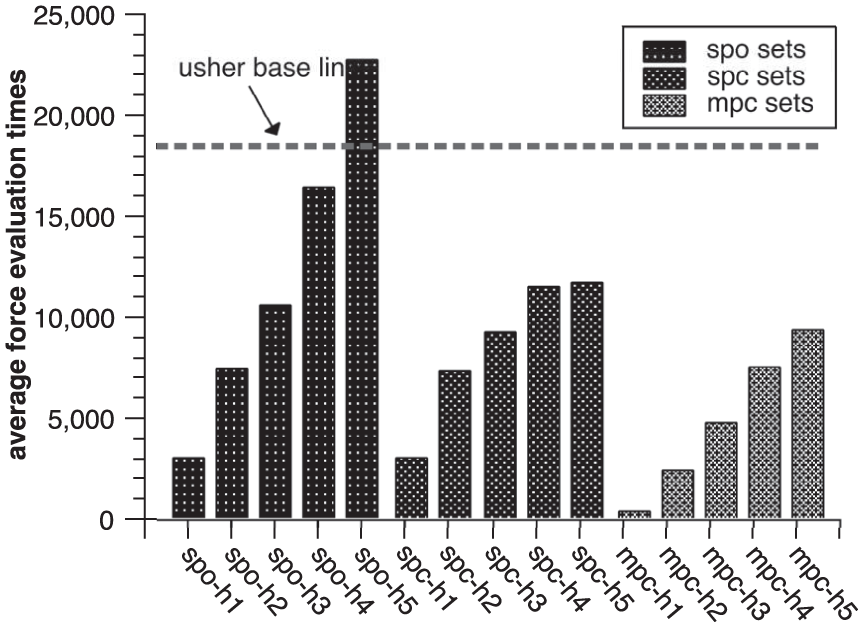
We present our WI-USHER algorithm superiority over the USHER algorithm under parallelism imbalance circumstance. The degree of parallelism is 12 and the MD domain is decomposed into 4 × 3, that is, four in the x-direction and three in y-direction, only four processes are inserted processes to accomplish the particle insertion operation. We show the average force evaluation times in Figure 20, the evaluation error in Figure 21, and the detailed time-consuming in Figure 22.

Figure 20.

Average force evaluation times for the WI-USHER algorithm with three exclusive rules, SPO, SPC, and MPC, and the result of the USHER algorithm is as the base line.

Figure 21.

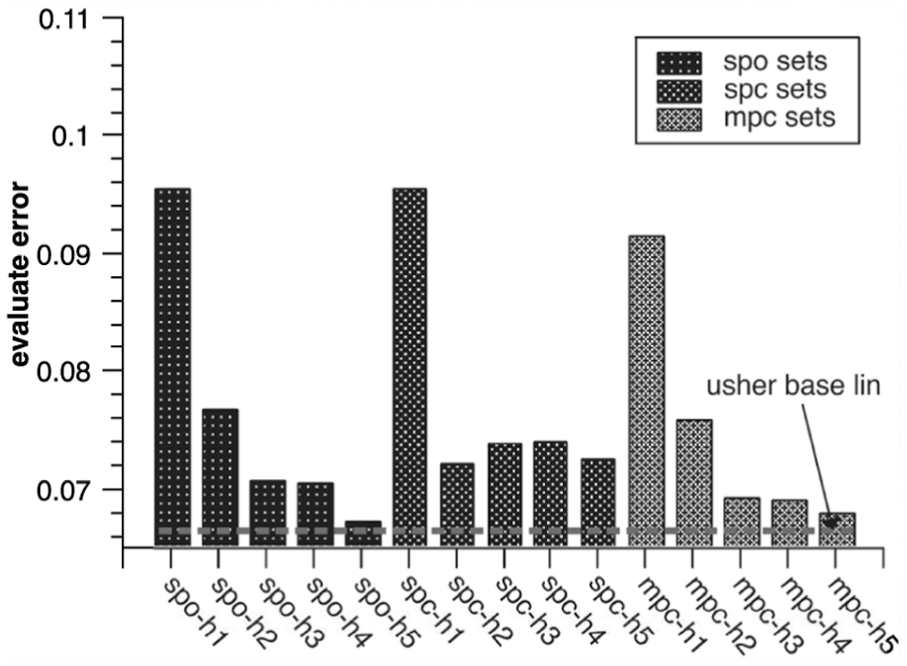
Average evaluation error for the WI-USHER algorithm with three exclusive rules, SPO, SPC, and MPC, and the result of USHER is as the base line.

Figure 22.

Detailed insertion time info, total simulation time, and data maintenance time of the WI-USHER algorithm.

The average force evaluation times of the USHER algorithm is 25,715 and the percentage of the particle insertion processing the total simulation time is 23.5%. The WI-USHER algorithm performs far superior to the USHER algorithm and the percentage decreases to only 3% of the total simulation time. The substantial decrease in the average force evaluation times leads to the alleviation of the imbalance of parallel particle insertion. We list the detailed percentage in Table 7, taking SPC-h3 as an example.

Table 7.

Detailed of parallel time-consuming.

	$t_{CFD}$ (percentage)	$t_{MD}$ (percentage)	$t_{CO}$ (percentage)	$t_{PI}$ (percentage)
USHER	47.03 (3.59)	862.49 (65.99)	397.46 (30.5)	307.08 (23.5)
SPC-h3	46.16 (4.46)	865.25 (83.6)	123.56 (11.93)	33.14 (3.19)

Worst case

The original USHER algorithm uses the local potential landscape to efficiently find the target position and performs superiority over our WI-USHER algorithm when the number density among moderate values. The reason is that the WI-USHER algorithm needs to maintain the relationship between particles and finer grids, and after excluding particle grids, the WI-USHER algorithm traverses all the remained grids to find the target position. When the number density is moderate, there are multi possible positions that meeting the target, the USHER algorithm that totally random chooses initial position performs better. We use Table 8 to describe the worse circumstance of our WI-USHER algorithm. Under the same simulation condition as in section “Periodic box,” we expect the number density to increasing from 0.4 to 0.6 within 200 insertions. The average force evaluation times, evaluation error, and detailed insertion time ( $t_{DM}$ , $t_{PI}$ ) are listed in Table 8. We can find that the USHER algorithm performs better than our WI-USHER algorithm under moderate number density.

Table 8.

Results of the worst case.

Method	Force evaluation times	Error	$t_{DM}$ (s)	$t_{PI}$ (s)
USHER	26.7	0.000722	0	0.0071
SPO	55.8	0.000741	0.0305	0.0386
SPC	53.3	0.00703	0.317	0.0398
MPC	56.6	0.000719	0.091	0.0987

Conclusions

The HAC method based on domain decomposition serves as an important tool for micro-fluid simulation, which obtains both simulation accuracy and efficiency. In HAC coupling method, mass exchanging between the continuum region and the atomistic region is one of the key operations to keep correct data exchanging between the two simulation methods. In order to deal with the mass exchanging, the particle insertion algorithm was proposed to handle the transformation for macroscopic velocity to number of insertion particles. For dense micro-fluid simulation, there exists a certain degree of parallelism load imbalance when directly using the USHER algorithm in the HAC coupling simulation. As we have tested the efficiency of the USHER algorithm, when the density in the inserted region reaches a slight high to high value, the iteration times of the USHER algorithm tend to reach a sufficient high value which brings in the imbalance between different inserted processes. There is an urgent need to improve the efficiency of particle insertion algorithm to reduce its operation time during the coupling simulation to balancing the insertion workload between processes. The optimization efficiency of the particle insertion algorithm will further improve the total simulation efficiency of the HAC method.

In this article, we propose a grid-based parallel particle insertion algorithm, named WI-USHER. The idea of the algorithm is, first, slicing the region to be inserted into finer grids with proper spacing scale, second, marking grids in black according to the occupation between particles and grids, the SPC of neighbor grids and the MPC of neighbor girds and third, using a steepest decent method to find the target insertion point. We implement our HAC coupling framework based on OpenFOAM and LAMMPS as well as the WI-USHER algorithm. We use two test cases to show the superiority of our WI-USHER algorithm over the USHER algorithm. Using three exclusive rules and proper finer grid slicing, the WI-USHER algorithm performs lower averaged force evaluation times, which decreases from $O (10^{4})$ to $O (10^{3})$ compared to the USHER algorithm. Furthermore, the percentage of the total simulation time processed by the particle insertion operation decreases from 23.5% to 3% compared to the USHER algorithm.

We aim to provide more comprehensive implementation of our WI-USHER algorithm for optimization of parameters to further improve the efficiency and workload balancing.

Footnotes

Academic Editor: Xiaotun Qiu

Declaration of conflicting interests

The author(s) declared no potential conflicts of interest with respect to the research, authorship, and/or publication of this article.

Funding

The author(s) disclosed receipt of the following financial support for the research, authorship, and/or publication of this article: The authors would like to thank the National Key Research and Development Program of China (No. 2016YFB0201301), Science Challenge Project (No. JCKY2016212A502), and the open fund from the State Key Laboratory of High Performance Computing (Grant No. 201303-01, 201503-01, and 201503-02).

References

Squires

Quake

SR.

Microfluidics: fluid physics at the nanoliter scale. Rev Mod Phys 2005; 77: 977–1026.

Whitesides

GM.

The origins and the future of microfluidics. Nature 2006; 442: 368–373.

Manz

Harrison

Verpoorte

. Planar chips technology for miniaturization and integration of separation techniques into monitoring systems: capillary electrophoresis on a chip. J Chromatogr A 1992; 593: 253–258.

Mohamed

Mohamad

AA.

A review of the development of hybrid atomistic-continuum methods for dense fluids. Microfluid Nanofluid 2010; 8: 283–302.

O’Connell

Thompson

PA.

Molecular dynamics–continuum hybrid computations: a tool for studying complex fluid flows. Phys Rev E 1995; 52: R5792–R5795.

Delgado-Buscalioni

Coveney

PV.

Usher: an algorithm for particle insertion in dense fluids. J Chem Phys 2003; 119: 978–987.

Fabritiis

Delgado-Buscalioni

Coveney

PV.

Energy controlled insertion of polar molecules in dense fluids. J Chem Phys 2004; 121: 12139–12142.

Borg

Lockerby

Reese

JM.

The FADE mass-stat: a technique for inserting or deleting particles in molecular dynamics simulations. J Chem Phys 2014; 140: 074110.

Wang

. Coupling strategies investigation of hybrid atomistic-continuum method based on state variable coupling. Adv Mater Sci Eng 2016.

10.

OpenFOAM. OpenFOAM, 2016, http://www.openfoam.org

11.

Plimpton

Fast parallel algorithms for short-range molecular dynamics. J Comput Phys 1995; 117: 1–19.

12.

Kalweit

Drikakis

Multiscale methods for micro/nano flows and materials. J Comput Theor Nanos 2008; 5: 1923–1938.

13.

Teschner

Knzsy

Jenkins

KW.

Progress in particlebased multiscale and hybrid methods for flow applications. Microfluid Nanofluid 2016; 20: 1–38.

14.

Zou

Yuan

Yang

. An integrated lattice Boltzmann and finite volume method for the simulation of viscoelastic fluid flows. J Non-Newton Fluid 2014; 211: 99–113.

15.

Guo

Wang

. A hybrid decomposition parallel algorithm for multi-scale simulation of viscoelastic fluids. In: 30st IEEE international parallel & distributed processing symposium, Chicago, IL, 23–27 May 2016. New York: IEEE.

16.

Neumann

Flohr

Arora

. Mamico: software design for parallel molecular-continuum flow simulations. Comput Phys Commun 2016; 200: 324–335.

17.

Nie

Chen

. A continuum and molecular dynamics hybrid method for micro- and nano-fluid flow. J Fluid Mech 2004; 500: 55–64.

18.

Werder

Walther

Koumoutsakos

Hybrid atomistic–continuum method for the simulation of dense fluid flows. J Comput Phys 2005; 205: 373–390.

19.

Johnson

Zollweg

Gubbins

KE.

The Lennard-Jones equation of state revisited. Mol Phys 1993; 78: 591–618.

20.

Voronoi

Nouvelles applications des paramètres continus à la théorie des formes quadratiques: deuxième mèmoire: recherches sur les parallélloèdres primitifs. J Für Diereine Angewandte Mathematik 1908; 134: 198–287.

21.

Lee

Cho

Lee

. A stochastic search approach for the multidimensional largest empty sphere problem, 2004.

22.

Shi

Yoshitsugu

A DC approach to the largest empty sphere problem in higher dimension. Berlin: Springer, 1996, pp.395–411.

23.

Strobl

Formella

Pschel

Exact calculation of the overlap volume of spheres and mesh elements. J Comput Phys 2016; 311: 158–172.

24.

Guo

Cao

. Multi-scale simulation of non-equilibrium phase transitions under shear flow in dilute polymer solutions. RSC Adv 2015; 5: 54649–54657.

25.

Huang

Statistical mechanics. New York: Wiley, 1987.

26.

Sun

Tao

. Roughness effect on flow and thermal boundaries in microchannel/nanochannel flow using molecular dynamics-continuum hybrid simulation. Int J Numer Meth Eng 2012; 89: 2–19.

WI-USHER: A grid-based parallel algorithm for particle insertion in hybrid atomistic-continuum method