On the dynamical motion of a gyro in the presence of external forces

Abstract

This work shed light on the motion of a symmetric rigid body (gyro) about one of its principal axes in the presence of a Newtonian force field besides a gyro moment in which its second component equals null. It is assumed that the body center of mass is shifted slightly relative to the dynamic symmetry axis. The governing equations of motion are investigated taking into account some initial conditions. The desired solutions of these equations are achieved in framework of the small parameter method. The periodic solutions for the case of irrational frequencies are investigated. Euler’s angles have been used to interpret the motion at any time. The geometrical representations of the obtained solutions and the phase plane schemas of these solutions are announced during several plots. Discussion of the results is presented to reinforce the importance of the considered gyro moment and the Newtonian force field. The significance of this problem is due to the framework of its several applications in different industries such as airplanes, submarines, compasses, spaceships, and guided missiles.

Introduction

The search for the analytical solutions of the rigid body problem about one of its fixed points is an important task in analytical mechanics. Generally, these kinds of problems required more complicated techniques because the governing system consists of six nonlinear differential equations in addition to three famous first integral.^1,2 It is known that, in order to obtain the solutions of like systems exactly, we need an algebraic complementary fourth first integral. Many researchers focused their works to realize such integrals,^3–8 whether in the case of gravitational force or in the presence of a Newtonian field or in the case of the motion under the action of a magnetic field or even under the effectiveness of a potential one. These trials require some restrictions on the center of mass and on the main moments of inertia.

The periodic solutions for the rotational motion of a rigid body under the influence of a Newtonian field of force were obtained in Ismail ⁹ using Krylov-Bogoliubov-Mitropolski technique. ¹⁰ The obtained solutions have singular points when the nature frequency equals integer numbers or its multiple inverse. Some of these singularities were treated in Ismail. ¹¹

In Amer et al., ¹² the same previous technique is modified to obtain the required solutions for the governing system of motion for a heavy solid spinning about one of the main axes of ellipsoid of inertia with high angular velocity. The rotation of this body is considered under the effectiveness of the gyro moment when its first component vanishes. The obtained solutions have no singular points at all because the authors used another frequency which differs from the natural frequency by a small quantity.

The exact solutions for the rigid body motion in the presence of external torque are presented in Romano ¹³ and extended in Romano ¹⁴ when two principal moments of inertia are equal to each other and the body moves under a constant external moment. Several publications have investigated the approximate solutions for the rigid body problem.^15–20 Longuski and colleagues^15,16 obtained the analytical approximate solutions using asymptotic and series expansion when the torque is equal a constant and when varies with time. Also, the rotational motion of a body undergoes a constant torque which was investigated by Livneh and Wie. ¹⁷ The solutions of this problem close to the equilibrium points undergo a Newtonian field of force are achieved in El-Sabaa. ²⁰

The method of small parameter^10,21 is used to investigate a class of solutions for special cases in Demin and Kiselev.^22,23 This advantage of the technique is used in Elfimov ¹⁸ to search for the existence of periodic solutions for the motion of a rigid body. The author supposed that the center of mass is slightly shifted from a dynamically symmetric axis. This problem was treated in Amer ¹⁹ when the body rotates under the action of nonzero components of the gyrostatic moment vector.

The task of this work is to investigate the rotational motion of a symmetric rigid body (gyro) under the effectiveness of a Newtonian field of force and undergo the gyrostatic moment vector in which its second component equals zero. The governing equations of motion are investigated after the imposition that the body center of mass is shifted slightly through a small quantity relative to the dynamical axis of symmetry in which this quantity is utilized to introduce a small parameter. The desired solutions of these equations are achieved applying the small parameter method of Poincaré, taking into account some certain initial conditions. The periodic solutions for the case of irrational frequencies are studied. These solutions are interpreted geometrically in framework of Euler’s angles to estimate the motion during any period of time. Interpretation and discussion of the results are presented to show the perfect effect of both the Newtonian field and the gyrostatic moment on the mentioned motion. Applications of this problem have a wide range in different industries, because the rigid body is considered as an appropriate model of numerous applications in life such as manipulators, spacecrafts, submarines, and compasses.

Description of the problem and the proposed method

Let O be a fixed point of a symmetric rigid body (gyro) about which the body rotates and takes place under the activity of a Newtonian field of force, arises from an attracting center subjected at point $O_1$ , and a gyrostatic moment $\underset{¯}{\ell }$ acting about the axes of rotation. Bearing in mind that the second component vanishes and the other two ones are different from zero. Let OXYZ be a fixed frame, in which $O_1$ lies on the downward Z-axis at a distance $R=O{O}_1$ and another one Oxyz, fixed in the body and moving with it in which its axes are directed along the main axes of the gyro at O (see Figure 1).

Figure 1.

Symmetric rigid body diagram.

One of the important aspects is to obtain the equations of motion of this problem. Euler–Poisson’s equations provided us with these equations. Moreover, the governing equations of motion can be obtained from the basic equation of the angular momentum which states that the rate of change of the angular momentum with respect to time t of a rigid body equals to the moments of all external forces acting on it, and from the directional cosines of the Z-axis with respect to the principle axes. So, the governing equations of motion have the following form ¹

$$\begin{array}{l}A\stackrel{.}{p}-(B-C)qr+q{\ell }_3-r{\ell }_2\\ =Mg(\gamma ″y_G-\gamma \prime z_G)-N(B-C)\gamma \prime \gamma ″\\ \stackrel{.}{\gamma }=r\gamma \prime -q\gamma ″;(p,q,r),(A,B,C),\\ (1,2,3),(x_G,y_G,z_G),(\gamma ,\gamma \prime ,\gamma ″)\end{array}$$

(1)

where $(A,B,C)$ represents the main moments of inertia, $(x_G,y_G,z_G)$ are the appropriate components of the body center of mass, $(p,q,r)$ are the components of angular velocity, $(\gamma ,\gamma \prime ,\gamma ″)$ denote the components of the unit vector along Z-axis direction into the axes of inertia, the over dots denote the derivatives with respect time t, M is the gyro’s mass, g is the gravitational acceleration, and $N=3\lambda /R^3$ , in which $\lambda$ is the constant of the attracting center $O_1$ .

Moreover, it is predicted that the other equations of motion can be obtained from equation (1) by the cyclic change of the symbols $(p,q,r),(A,B,C),(1,2,3)$ , $(x_G,y_G,z_G)$ , and $(\gamma ,\gamma \prime ,\gamma ″)$ .

After some algebraic manipulations and with the aid of the previous equations, one obtains the three first integrals, namely, energy integral, area integral, and geometric ones in the following form ¹

$$\begin{array}{l}A{p}^2+B{q}^2+C{r}^2-2Mg(\gamma x_G+\gamma \prime y_G+\gamma ″z_G)+N(A{\gamma }^2+B\gamma {\prime }^2\\ +C{\gamma ″}^2)=A{p}_0^2+B{q}_0^2+C{r}_0^2-2Mg({\gamma }_0{x}_G+\gamma {\prime }_0{y}_G+\gamma \prime {\prime }_0{z}_G)\\ +N(A{\gamma }_0^2+B\gamma {\prime }_0^2+C\gamma \prime {\prime }_0^2)\\ (Ap+{\ell }_1)\gamma +Bq\gamma \prime +(Cr+{\ell }_3)\gamma ″=(A{p}_0+{\ell }_1){\gamma }_0+B{q}_0\gamma {\prime }_0\\ +(C{r}_0+{\ell }_3)\gamma \prime {\prime }_0\\ {\gamma }^2+\gamma {\prime }^2+{\gamma ″}^2=1\end{array}$$

(2)

where $p_0,q_0,r_0,{\gamma }_0,\gamma {\prime }_0$ , and ${\gamma ″}_0$ are the initial values of their corresponding variables.

Taking into consideration that the body is symmetric about one of its principal axes, the second component of gyrostatic moment equals null, and the center of mass is shifted slightly (to some extent) relative to the axis of dynamical symmetry. This small displacement has been used to introduce the small dimensionless parameter $ϵ$ . Consequently, to visualize the motion, we consider that

$$x_G=\sqrt{ϵ}{z}_G,y_G=0,A=B\ne C,$$

in order to obtain the following dimensionless quantities

$$\begin{array}{c}p=\sqrt{ϵ}\frac{p_1}{n},q=\sqrt{ϵ}\frac{q_1}{n},r=\frac{r_1}{n},\gamma =\sqrt{ϵ}{\gamma }_1\hfill \\ \gamma \prime =\sqrt{ϵ}{\gamma \prime }_1,\gamma ″={\gamma ″}_1,{\ell }_1=\frac{A}{n}\sqrt{ϵ}{\ell \prime }_1,{\ell }_3=\frac{A}{n}{\ell \prime }_3\hfill \\ t=n\tau ,n=\sqrt{\frac{A}{\mathrm{Mg}{z}_G}},k=\mathrm{Na}{n}^2,\hfill \\ a=\frac{(A-C)}{A},b=\frac{C}{A}\hfill \end{array}$$

(3)

Inserting the previous assumptions and the substitutions (3) into the system of equations (1) and the first integrals (2), we obtain

$$\begin{array}{c}\frac{d{p}_1}{d\tau }=a{q}_1{r}_1-q_1{\ell \prime }_3-{\gamma \prime }_1-k{\gamma \prime }_1{\gamma ″}_1\hfill \\ \frac{d{q}_1}{d\tau }=-a{r}_1{p}_1+p_1{\ell \prime }_3-r_1{\ell \prime }_1+{\gamma }_1-{\gamma ″}_1+k{\gamma }_1{\gamma ″}_1\hfill \\ \frac{d{r}_1}{d\tau }=\epsilon (q_1{\ell \prime }_1+b^{-1}{\gamma \prime }_1)\hfill \\ \frac{d{\gamma }_1}{d\tau }=r_1{\gamma \prime }_1-q_1{\gamma ″}_1,\frac{d{\gamma \prime }_1}{d\tau }=p_1{\gamma ″}_1-r_1{\gamma }_1\hfill \\ \frac{d{\gamma ″}_1}{d\tau }=ϵ(q_1{\gamma }_1-p_1{\gamma \prime }_1)\hfill \end{array}$$

(4)

and

$$\begin{array}{c}ϵ(p_1^2+q_1^2-2{\gamma }_1)+{\mathrm{br}}_1^2-2{\gamma ″}_1-k{\gamma ″}_1^2\hfill \\ =ϵ(p_{10}^2+q_{10}^2-2{\gamma }_{10})\hfill \\ +{\mathrm{br}}_{10}^2-2{\gamma ″}_{10}-k{\gamma }_{10}^{″2}\hfill \\ ϵ[(p_1+{\ell \prime }_1){\gamma }_1+q_1{\gamma \prime }_1]+(b{r}_1+{\ell \prime }_3){\gamma ″}_1\hfill \\ =ϵ[(p_{10}+{\ell \prime }_1){\gamma }_{10}+q_{10}{\gamma \prime }_{10}]\hfill \\ +(b{r}_{10}+{\ell \prime }_3){\gamma ″}_{10}\hfill \\ ϵ({\gamma }_1^2+{\gamma }_1^{\prime 2})+{\gamma }_1^{″2}=1\hfill \end{array}$$

(5)

In order to reduce system (4) to another appropriate one, ${\gamma ″}_1$ and $r_1$ can be obtained from the third and first equations of (5) as

$$\begin{array}{c}{\gamma ″}_1=1-ϵf_1,r_1=r_{10}-ϵf_2\hfill \end{array}$$

(6)

where

$$\begin{array}{c}{f}_1=\frac{1}{2}{F}_1+\frac{ϵ}{8}{F}_1^2+\cdots ,F_1={\gamma }_1^2+{\gamma }_1^{\prime 2}\hfill \\ f_2=\frac{1}{2b{r}_{10}}(F_2-F_{20})+\frac{ϵ}{8b{r}_{10}}(F_1^2-F_{20}^2)\hfill \\ +\frac{{ϵ}^2}{8b^2{r}_{10}^3}{(F_2-F_{20})}^2+\cdots ,\hfill \\ F_2=p_1^2+q_1^2-2{\gamma }_1+F_1(k+1)\hfill \end{array}$$

(7)

where $F_{10}$ and $F_{20}$ are the initial values of $F_1$ and $F_2$ respectively.

Now, using equations (6) and omitting ${\gamma ″}_1$ and $r_1$ from system (4), we obtain another system consisting of four nonlinear first-order differential equations, and then use the following new substitutions ¹⁹

$$\begin{array}{c}{p}_1=p_2+h{\gamma }_2+C_1,{\gamma }_1=(1+\beta h){\gamma }_2+\beta p_2+C_2\hfill \\ q_1=q_2+h{\gamma \prime }_2,{\gamma \prime }_1=(1+\beta h){\gamma \prime }_2+\beta q_2\hfill \end{array}$$

(8)

to transform system (4) to the following more convenient form

$$\begin{array}{c}\frac{d{p}_2}{d\tau }={\lambda }_1{q}_2+ϵG_1,\frac{d{q}_2}{d\tau }=-{\lambda }_1{p}_2+ϵG_2\hfill \\ \frac{d{\gamma }_2}{d\tau }={\lambda }_2{\gamma \prime }_2+ϵG_3,\frac{d{\gamma \prime }_2}{d\tau }=-{\lambda }_2{\gamma }_2+ϵG_4\hfill \end{array}$$

(9)

where

$$\begin{array}{c}h=-\frac{(1+k)}{\pm \sqrt{{(b{r}_{10}+{\ell \prime }_3)}^2+4(1+k)}},C_1=\frac{r_{10}(1+{\ell \prime }_3{r}_{10})}{(1+k+r_{10}{\ell \prime }_3-{\mathrm{ar}}_{10}^2)}\hfill \\ \beta =\frac{[-(b{r}_{10}+{\ell \prime }_3)\pm \sqrt{{(b{r}_{10}+{\ell \prime }_3)}^2+4(1+k)}]}{2(1+k)},C_2=\frac{C_1}{r_{10}}\hfill \\ {\lambda }_1=h(1-\beta r_{10})+(1+\beta h)[a{r}_{10}-\beta (1+k)-{\ell \prime }_3]\hfill \\ {\lambda }_2=-h(1+\beta a{r}_{10})+(1+\beta h)[r_{10}+\beta (1+k)]+\beta h{\ell \prime }_3\hfill \\ G_1=h(f_2{\gamma \prime }_2-q_1{f}_1)-(1+\beta h)(a{f}_2{q}_1-k{f}_1{\gamma \prime }_1)\hfill \\ G_2=h(f_1{p}_1-f_2{\gamma }_1)+(1+\beta h)[f_2(a{p}_1+{\ell \prime }_1)+f_1(1-k{\gamma }_1)]\hfill \\ G_3=\beta (a{f}_2{q}_1-k{f}_1{\gamma \prime }_1)-(f_2{\gamma \prime }_1-q_1{f}_1)\hfill \\ G_4=-\beta [f_1(1-k{\gamma }_1)+f_2(a{p}_1+{\ell \prime }_1)]-(f_1{p}_1-f_2{\gamma }_1)\hfill \end{array}$$

(10)

It is worthwhile to note that with a suitable selection of $r_0$ , the division of the frequency ${\lambda }_1$ over ${\lambda }_2$ can be considered as a rational number. This elucidates that the solution of the generating system of system (9) is then periodic with period $(T_0=2\pi n_v/{\lambda }_v;v=1,2)$ . Let us reformulate the problem that determines ${\tau }_0(ϵ)$ -periodic solutions of system (9) with a very small value of $ϵ$ , which for $ϵ=0$ would transform to a solution of period $T_0$ of system (9) at $ϵ=0$ . So, let us consider $\tau =(1+ϵ\alpha )T$ , where $\alpha$ is a function of $ϵ$ that can be determined. The problem is now transformed to determine the periodic solutions with period $T_0$ to the following system

$$\begin{array}{c}\frac{d{p}_2}{\mathrm{dT}}={\lambda }_1{q}_2+ϵH_1,\frac{d{q}_2}{\mathrm{dT}}=-{\lambda }_1{p}_2+ϵH_2\hfill \\ \frac{d{\gamma }_2}{\mathrm{dT}}={\lambda }_2{\gamma \prime }_2+ϵH_3,\frac{d{\gamma \prime }_2}{\mathrm{dT}}=-{\lambda }_2{\gamma }_2+ϵH_4\hfill \end{array}$$

(11)

where

$$\begin{array}{c}{H}_1={\lambda }_1\alpha q_2+(1+ϵ\alpha )G_1,H_2=-{\lambda }_1\alpha p_2+(1+ϵ\alpha )G_2\hfill \\ H_3={\lambda }_2\alpha {\gamma \prime }_2+(1+ϵ\alpha )G_3,H_4=-{\lambda }_2\alpha {\gamma }_2+(1+ϵ\alpha )G_4\hfill \\ H_i=H_i^{(1)}+ϵH_i^{(2)}+{ϵ}^2{H}_i^{(3)}+\cdots \hfill \end{array}$$

(12)

Differentiating system (11) with respect to T and using again system (11), one obtains another one which consists of four differential equations from second order. In view of the resulted equations, one can seek the desired periodic solutions in the form

$$\begin{array}{c}{p}_2(T,ϵ)=M_1\cos {\lambda }_{1}T+M_2\sin {\lambda }_{1}T+\sum _1\hfill \\ \multicolumn{1}{c}{q_2(T,ϵ)=-M_1\sin {\lambda }_{1}T+M_2\cos {\lambda }_{1}T+\sum _2}\\ \multicolumn{1}{c}{{\gamma }_2(T,ϵ)=M_3\cos {\lambda }_{2}T+\sum _3}\\ \multicolumn{1}{c}{{\gamma \prime }_2(T,ϵ)=-M_3\sin {\lambda }_{2}T+\sum _4}\\ \multicolumn{1}{c}{\sum _i=\sum _{n=1}^{\infty }{ϵ}^n{C}_i^{(n)},i=1,2,3,4}\end{array}$$

(13)

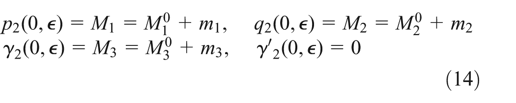
besides the following initial conditions

$$\begin{array}{c}{p}_2(0,ϵ)=M_1=M_1^0+m_1,q_2(0,ϵ)=M_2=M_2^0+m_2\hfill \\ \multicolumn{1}{c}{{\gamma }_2(0,ϵ)=M_3=M_3^0+m_3,{\gamma \prime }_2(0,ϵ)=0}\end{array}$$

(14)

Here, $(M_j^{(0)};j=1,2,3)$ are the unperturbed terms in $M_j$ and we seek $(m_i;i=1,2,3,4)$ as functions of $ϵ$ such that it equals zero when $ϵ$ vanishes.

From the inspection of system (9), it is clear that the periodic solutions of this system, which correspond to the $T_0$ -periodic solutions of system (11), are of period $T_1=(1+ϵ\alpha )T_0$ which for $ϵ=0$ reduces to the period of the generating system $(2\pi n_v/{\lambda }_v;v=1,2)$ . We assume that $\alpha ={\alpha }_0+m_4$ . In harmony with the small parameter method, the initial conditions can be varied to correspond with the arbitrary constants of solutions of the generating system. We also vary $\alpha$ to have periodic solutions for (13).

Substituting $p_1,q_1,{\gamma }_1$ , and $\gamma {\prime }_1$ from (8) into (7), one gets $F_1^{(0)}$ and $F_2^{(0)}$ in terms of $\cos {\lambda }_{v}T$ and $\sin {\lambda }_{v}T;(v=1,2)$ .

Making use of equations (8) and (10), reformulate $(G_i;i=1,2,3,4)$ in short forms as follows

$$\begin{array}{c}{G}_1=L_1{q}_2+L_2{\gamma \prime }_2,G_2=-(L_1{p}_2+L_2{\gamma }_2)+L_3\hfill \\ \multicolumn{1}{c}{G_3=L_4{q}_2+L_5{\gamma \prime }_2,G_4=-(L_4{p}_2+L_5{\gamma }_2)+L_6}\end{array}$$

(15)

where

$$\begin{array}{c}{L}_1=(1+\beta h)(k\beta f_1-a{f}_2)+h(\beta f_2-f_1)\hfill \\ L_2=(1+\beta h)[(1+\beta h)k{f}_1+h{f}_2(1-a)]-h^2{f}_1\hfill \\ L_3=(1+\beta h)[(a{C}_1+{\ell \prime }_1)f_2+f_1(1-k{C}_2)]+h(C_1{f}_1-C_2{f}_2)\hfill \\ L_4=\beta f_2(a-1)+f_1(1-k{\beta }^2)\hfill \\ L_5=h(a\beta f_2+f_1)-(1+\beta h)(f_2+k\beta f_1)\hfill \\ L_6=-\beta [(a{C}_1+{\ell \prime }_1)f_2+f_1(1-k{C}_2)]-(C_1{f}_1-C_2{f}_2)\hfill \end{array}$$

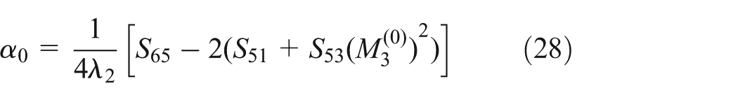
Under the present circumstances, eliminate the independent terms of $ϵ$ in $(L_s;s=1,2,\dots ,6)$ to obtain the following form

$$\begin{array}{c}\multicolumn{1}{c}{L_i^{(0)}=[S_{i1}+S_{i2}(M_1^2+M_2^2)+S_{i3}{M}_3^2]+S_{i4}(M_1}\\ \times \cos {\lambda }_{1}T+M_2\sin {\lambda }_{1}T)+S_{i5}{M}_3\cos {\lambda }_{2}T\hfill \\ +S_{i6}{M}_3[M_1\cos ({\lambda }_1-{\lambda }_2)T+M_2\sin ({\lambda }_1-{\lambda }_2)T]\hfill \end{array}$$

(16)

where $S_{\mathrm{ij}}$ represents a matrix of constant coefficients $(\parallel S_{\mathrm{ij}}\parallel ;i,j=1,2,\dots ,6)$ . Moreover, to obtain these coefficients, it is necessary to determine $f_1^{(0)}$ and $f_2^{(0)}$ . For this purpose, using the forms of $F_1^{(0)},F_2^{(0)}$ , and equations (7) to obtain $f_1^{(0)}$ and $f_1^{(0)}$ . Consequently, one obtains easily $(S_{1j},S_{2j},\dots ,S_{6j};j=1,2,\dots ,6)$ (see Appendix 1).

Substituting from the desired solutions (13) into system (11), equating the coefficients of like powers of $ϵ$ and then the coefficients $C_i^{(n)}(T)$ can be determined by the following equations

$$\begin{array}{l}\frac{d{C}_1^{(n)}}{dT}={\lambda }_1{C}_2^{(n)}(T)+H_1^{(n)}(T)\\ \frac{d{C}_2^{(n)}}{dT}=-{\lambda }_1{C}_1^{(n)}(T)+H_2^{(n)}(T)\\ \frac{d{C}_3^{(n)}}{dT}={\lambda }_{2}d{C}_4^{(n)}(T)+H_3^{(n)}(T)\\ \frac{d{C}_4^{(n)}}{dT}=-{\lambda }_2{C}_3^{(n)}(T)+H_4^{(n)}(T)\end{array}$$

(17)

in addition to the initial conditions $(C_i^{(n)}(0)=0;i=1,2,3,4)$ . Here, $H_i^{(n)}(T)$ are the known functions if $C_i^{(j)}(T)$ is determined for $j<n$ .

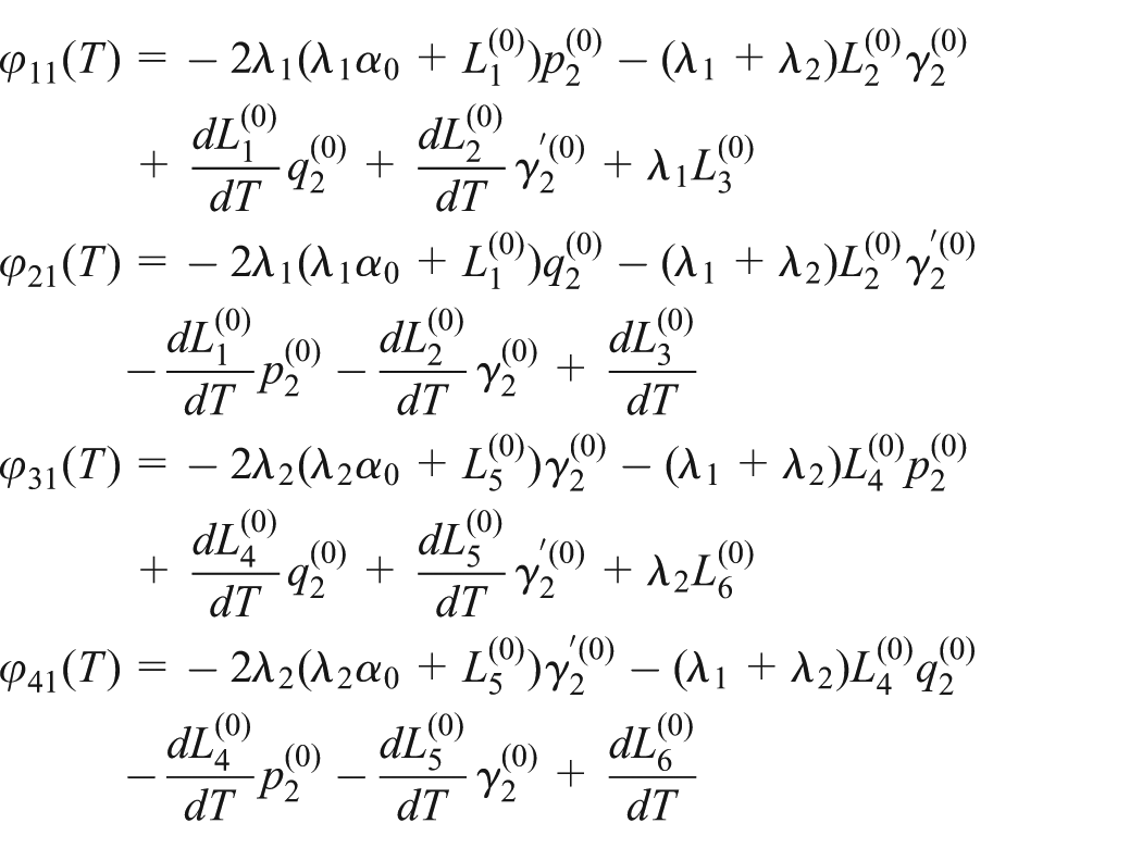
For $n=1$ , substituting (12) into system of equations (17), equating the coefficients of equal powers of $ϵ$ and then differentiating the resulting equations with respect to T, one obtains equations determining $(C_i^{(1)}(T);i=1,2,3,4)$ in the following form

$$\begin{array}{c}\frac{d^2{C}_1^{(1)}}{d{T}^2}+{\lambda }_1^2{C}_1^{(1)}(T)={\phi }_{11}(T)\hfill \\ \frac{d^2{C}_2^{(1)}}{d{T}^2}+{\lambda }_1^2{C}_2^{(1)}(T)={\phi }_{21}(T)\hfill \\ \frac{d^2{C}_3^{(1)}}{d{T}^2}+{\lambda }_2^2{C}_3^{(1)}(T)={\phi }_{31}(T)\hfill \\ \frac{d^2{C}_4^{(1)}}{d{T}^2}+{\lambda }_2^2{C}_4^{(1)}(T)={\phi }_{41}(T)\hfill \end{array}$$

(18)

where

$$\begin{array}{c}{\phi }_{11}(T)=-2{\lambda }_1({\lambda }_1{\alpha }_0+L_1^{(0)})p_2^{(0)}-({\lambda }_1+{\lambda }_2)L_2^{(0)}{\gamma }_2^{(0)}\hfill \\ \multicolumn{1}{c}{+\frac{{\mathrm{dL}}_1^{(0)}}{\mathrm{dT}}{q}_2^{(0)}+\frac{{\mathrm{dL}}_2^{(0)}}{\mathrm{dT}}{\gamma }_2^{\prime (0)}+{\lambda }_1{L}_3^{(0)}}\\ \multicolumn{1}{c}{{\phi }_{21}(T)=-2{\lambda }_1({\lambda }_1{\alpha }_0+L_1^{(0)})q_2^{(0)}-({\lambda }_1+{\lambda }_2)L_2^{(0)}{\gamma }_2^{\prime (0)}}\\ \multicolumn{1}{c}{-\frac{{\mathrm{dL}}_1^{(0)}}{\mathrm{dT}}{p}_2^{(0)}-\frac{{\mathrm{dL}}_2^{(0)}}{\mathrm{dT}}{\gamma }_2^{(0)}+\frac{{\mathrm{dL}}_3^{(0)}}{\mathrm{dT}}}\\ \multicolumn{1}{c}{{\phi }_{31}(T)=-2{\lambda }_2({\lambda }_2{\alpha }_0+L_5^{(0)}){\gamma }_2^{(0)}-({\lambda }_1+{\lambda }_2)L_4^{(0)}{p}_2^{(0)}}\\ \multicolumn{1}{c}{+\frac{{\mathrm{dL}}_4^{(0)}}{\mathrm{dT}}{q}_2^{(0)}+\frac{{\mathrm{dL}}_5^{(0)}}{\mathrm{dT}}{\gamma }_2^{\prime (0)}+{\lambda }_2{L}_6^{(0)}}\\ \multicolumn{1}{c}{{\phi }_{41}(T)=-2{\lambda }_2({\lambda }_2{\alpha }_0+L_5^{(0)}){\gamma }_2^{\prime (0)}-({\lambda }_1+{\lambda }_2)L_4^{(0)}{q}_2^{(0)}}\\ \multicolumn{1}{c}{-\frac{{\mathrm{dL}}_4^{(0)}}{\mathrm{dT}}{p}_2^{(0)}-\frac{{\mathrm{dL}}_5^{(0)}}{\mathrm{dT}}{\gamma }_2^{(0)}+\frac{{\mathrm{dL}}_6^{(0)}}{\mathrm{dT}}}\end{array}$$

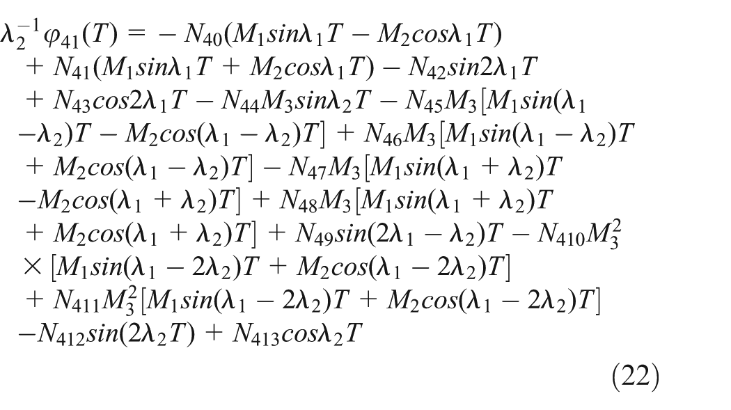
Having $({\phi }_{i1}(T);i=1,2,3,4)$ , one gets the solutions of system of equations (18) directly in the following form

$$\begin{array}{c}{C}_1^{(1)}(T)={\lambda }_1^{-1}{\int }_0^T{\phi }_{11}(u)\sin {\lambda }_1(T-u)\mathrm{du}\hfill \\ \multicolumn{1}{c}{C_2^{(1)}(T)={\lambda }_1^{-1}{\int }_0^T{\phi }_{21}(u)\sin {\lambda }_1(T-u)\mathrm{du}}\\ \multicolumn{1}{c}{C_3^{(1)}(T)={\lambda }_2^{-1}{\int }_0^T{\phi }_{31}(u)\sin {\lambda }_2(T-u)\mathrm{du}}\\ \multicolumn{1}{c}{C_4^{(1)}(T)={\lambda }_2^{-1}{\int }_0^T{\phi }_{41}(u)\sin {\lambda }_2(T-u)\mathrm{du}}\end{array}$$

(19)

where

$$\begin{array}{c}{\lambda }_1^{-1}{\phi }_{11}(T)=N_{10}+N_{11}(M_1\cos {\lambda }_{1}T+M_2\sin {\lambda }_{1}T)\hfill \\ \multicolumn{1}{c}{+N_{12}(M_1\cos {\lambda }_{1}T-M_2\sin {\lambda }_{1}T)+N_{13}\cos 2{\lambda }_{1}T}\\ \multicolumn{1}{c}{+N_{14}\sin 2{\lambda }_{1}T+N_{15}{M}_3\cos {\lambda }_{2}T+N_{16}{M}_3[M_1}\\ \multicolumn{1}{c}{\times \cos ({\lambda }_1-{\lambda }_2)T+M_2\sin ({\lambda }_1-{\lambda }_2)T]+N_{17}{M}_3}\\ \multicolumn{1}{c}{\times [M_1\cos ({\lambda }_1-{\lambda }_2)T-M_2\sin ({\lambda }_1-{\lambda }_2)T]}\\ \multicolumn{1}{c}{+N_{18}{M}_3[M_1\cos ({\lambda }_1+{\lambda }_2)T+M_2\sin ({\lambda }_1+{\lambda }_2)T]}\\ \multicolumn{1}{c}{-N_{15}{M}_3[M_1\cos ({\lambda }_1+{\lambda }_2)T-M_2\sin ({\lambda }_1+{\lambda }_2)T]}\\ \multicolumn{1}{c}{+N_{19}\cos (2{\lambda }_1-{\lambda }_2)T+N_{110}\sin (2{\lambda }_1-{\lambda }_2)T}\\ \multicolumn{1}{c}{+N_{111}{M}_3^2[M_1\cos ({\lambda }_1-2{\lambda }_2)T+M_2\sin ({\lambda }_1-2{\lambda }_2)T]}\\ \multicolumn{1}{c}{+N_{112}{M}_3^2[M_1\cos ({\lambda }_1-2{\lambda }_2)T-M_2\sin ({\lambda }_1-2{\lambda }_2)T]}\\ \multicolumn{1}{c}{+N_{113}\cos 2{\lambda }_{2}T}\end{array}$$

(20)

$$\begin{array}{c}{\lambda }_1^{-1}{\phi }_{21}(T)=-N_{20}(M_1\sin {\lambda }_{1}T-M_2\cos {\lambda }_{1}T)+N_{21}(M_1\sin {\lambda }_{1}T\hfill \\ +M_2\cos {\lambda }_{1}T)-N_{22}{M}_3\sin {\lambda }_{2}T-N_{23}{M}_3[M_1\sin ({\lambda }_1-{\lambda }_2)T\hfill \\ -M_2\cos ({\lambda }_1-{\lambda }_2)T]+N_{24}{M}_3[M_1\cos ({\lambda }_1-{\lambda }_2)T+M_2\sin ({\lambda }_1\hfill \\ -{\lambda }_2)T]+N_{25}{M}_3[M_1\sin ({\lambda }_1-{\lambda }_2)T+M_2\cos ({\lambda }_1-{\lambda }_2)T]\hfill \\ -N_{26}{M}_3[M_1\sin ({\lambda }_1+{\lambda }_2)T-M_2\cos ({\lambda }_1+{\lambda }_2)T]+N_{27}{M}_3\hfill \\ \times [M_1\sin ({\lambda }_1+{\lambda }_2)T+M_2\cos ({\lambda }_1+{\lambda }_2)T]+N_{28}\sin (2{\lambda }_1\hfill \\ -{\lambda }_2)T+N_{29}{M}_3^2[M_1\sin ({\lambda }_1-2{\lambda }_2)T+M_2\cos ({\lambda }_1-2{\lambda }_2)T]\hfill \\ +N_{210}{M}_3^2[M_1\sin ({\lambda }_1-2{\lambda }_2)T-M_2\cos ({\lambda }_1-2{\lambda }_2)T]\hfill \\ -N_{211}\sin 2{\lambda }_{2}T+N_{212}{M}_3\cos {\lambda }_{2}T\hfill \\ {\lambda }_2^{-1}{\phi }_{31}(T)=N_{30}+N_{31}{M}_3\sin {\lambda }_{2}T+N_{32}{M}_3\cos {\lambda }_{2}T\hfill \\ +N_{33}{M}_3^2\cos 2{\lambda }_{2}T\hfill \end{array}$$

(21)

$$\begin{array}{c}{\lambda }_2^{-1}{\phi }_{41}(T)=-N_{40}(M_1\sin {\lambda }_{1}T-M_2\cos {\lambda }_{1}T)\hfill \\ \multicolumn{1}{c}{+N_{41}(M_1\sin {\lambda }_{1}T+M_2\cos {\lambda }_{1}T)-N_{42}\sin 2{\lambda }_{1}T}\\ \multicolumn{1}{c}{+N_{43}\cos 2{\lambda }_{1}T-N_{44}{M}_3\sin {\lambda }_{2}T-N_{45}{M}_3[M_1\sin ({\lambda }_1}\\ \multicolumn{1}{c}{-{\lambda }_2)T-M_2\cos ({\lambda }_1-{\lambda }_2)T]+N_{46}{M}_3[M_1\sin ({\lambda }_1-{\lambda }_2)T}\\ \multicolumn{1}{c}{+M_2\cos ({\lambda }_1-{\lambda }_2)T]-N_{47}{M}_3[M_1\sin ({\lambda }_1+{\lambda }_2)T}\\ \multicolumn{1}{c}{-M_2\cos ({\lambda }_1+{\lambda }_2)T]+N_{48}{M}_3[M_1\sin ({\lambda }_1+{\lambda }_2)T}\\ \multicolumn{1}{c}{+M_2\cos ({\lambda }_1+{\lambda }_2)T]+N_{49}\sin (2{\lambda }_1-{\lambda }_2)T-N_{410}{M}_3^2}\\ \multicolumn{1}{c}{\times [M_1\sin ({\lambda }_1-2{\lambda }_2)T+M_2\cos ({\lambda }_1-2{\lambda }_2)T]}\\ \multicolumn{1}{c}{+N_{411}{M}_3^2[M_1\sin ({\lambda }_1-2{\lambda }_2)T+M_2\cos ({\lambda }_1-2{\lambda }_2)T]}\\ \multicolumn{1}{c}{-N_{412}\sin (2{\lambda }_{2}T)+N_{413}\cos {\lambda }_{2}T}\end{array}$$

(22)

Here, $(N_{1i};i=0,1,\dots ,13),(N_{2j};j=0,1,\dots ,12),(N_{3k};k=0,1,2),$ and $(N_{4v};v=0,1,\dots ,13)$ are constants and can be obtained directly (see Appendix 2). Substituting from equations (20), (21), and (22) into equations (19), we obtain

$$\begin{array}{c}{C}_1^{(1)}(T_0)=(E_{11}+R_{11})T_0;E_{11}=(N_{12}-N_{11})M_2/2\hfill \\ \multicolumn{1}{c}{C_2^{(1)}(T_0)=(E_{21}+R_{21})T_0;E_{21}=(N_{20}{M}_1-N_{21}{M}_2)/2}\\ \multicolumn{1}{c}{C_4^{(1)}(T_0=-(E_{31}+R_{41})T_0;E_{11}=-N_{42}{M}_3/2}\end{array}$$

(23)

It is remarked in Malkin ²¹ that for the solutions (13) to be $T_0$ -periodic, it is necessary and sufficient to realize the following periodicity conditions

$$\begin{array}{c}{\psi }_1=p_2(T_0,ϵ)-p_2(0,ϵ)=0,{\psi }_2=q_2(T_0,ϵ)-q_2(0,ϵ)=0\hfill \\ {\psi }_3={\gamma }_2(T_0,ϵ)-{\gamma }_2(0,ϵ)=0,{\psi }_4={\gamma \prime }_2(T_0,ϵ)-{\gamma \prime }_2(0,ϵ)=0\hfill \end{array}$$

(24)

where $({\psi }_i;i=1,2,3,4)$ are considered as functions of $(M_j;j=1,2,3),\alpha$ , and $ϵ$ . Equalities (24) that determine $M_j^0,{\alpha }_0$ , and $m_i$ are not independent due to the existence of the first integral in system (11). ¹⁸ Moreover, it is predicted that the third condition is a corollary of the remaining if $M_3\ne 0$ . According to the statement in Arkhangelskii, ²⁴ it is convenient to look one of the $M_j^0$ or ${\alpha }_0$ as a constant, and one of the $m_i$ as a function of $ϵ$ that vanishes when $ϵ=0$ .

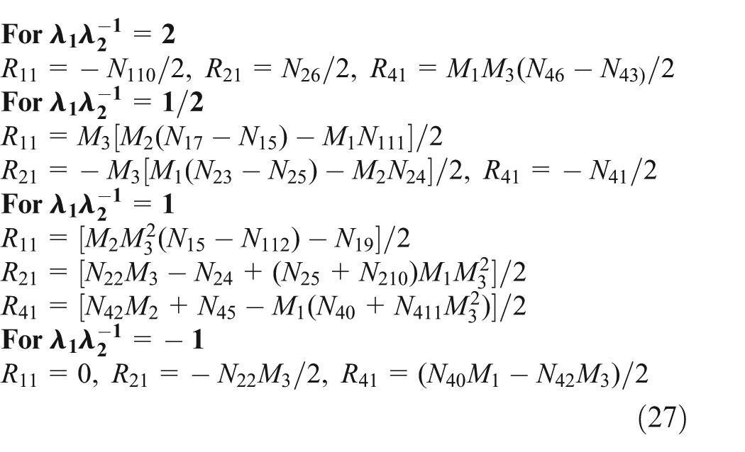
Reducing equalities (24) by $ϵ$ , and then equating the terms of zero powers of $ϵ$ with zero, to yield the necessary periodicity conditions

$$C_l^{(1)}(T_0)=C_l^{(1)}(M_1,M_2,M_3,\alpha );(l=1,2,4).$$

(25)

By analogy with equations (23), one gets

$$E_{11}+R_{11}=0,E_{21}+R_{21}=0,E_{31}+R_{41}=0.$$

(26)

It should be noted that if ${\lambda }_1{\lambda }_2^{-1}$ is equal to either of 2, 1/2, 1, or −1, the expressions of $R_{11},R_{21}$ , and $R_{41}$ do not vanish and take the following forms

$$\begin{array}{c}\mathbf{For}{\mathbf{\lambda }}_1{\mathbf{\lambda }}_2^{-1}=2\hfill \\ \multicolumn{1}{c}{R_{11}=-N_{110}/2,R_{21}=N_{26}/2,R_{41}=M_1{M}_3(N_{46}-N_{43)}/2}\\ \multicolumn{1}{c}{\mathbf{For}{\mathbf{\lambda }}_1{\mathbf{\lambda }}_2^{-1}=1/2}\\ \multicolumn{1}{c}{R_{11}=M_3[M_2(N_{17}-N_{15})-M_1{N}_{111}]/2}\\ \multicolumn{1}{c}{R_{21}=-M_3[M_1(N_{23}-N_{25})-M_2{N}_{24}]/2,R_{41}=-N_{41}/2}\\ \multicolumn{1}{c}{\mathbf{For}{\mathbf{\lambda }}_1{\mathbf{\lambda }}_2^{-1}=1}\\ \multicolumn{1}{c}{R_{11}=[M_2{M}_3^2(N_{15}-N_{112})-N_{19}]/2}\\ \multicolumn{1}{c}{R_{21}=[N_{22}{M}_3-N_{24}+(N_{25}+N_{210})M_1{M}_3^2]/2}\\ \multicolumn{1}{c}{R_{41}=[N_{42}{M}_2+N_{45}-M_1(N_{40}+N_{411}{M}_3^2)]/2}\\ \multicolumn{1}{c}{\mathbf{For}{\mathbf{\lambda }}_1{\mathbf{\lambda }}_2^{-1}=-1}\\ \multicolumn{1}{c}{R_{11}=0,R_{21}=-N_{22}{M}_3/2,R_{41}=(N_{40}{M}_1-N_{42}{M}_3)/2}\end{array}$$

(27)

Let $(M_j^{(0)};j=1,2,3)$ and ${\alpha }_0$ satisfy system (26), consider Jacobi’s matrices of $(C_l(T_0);l=1,2,4)$ in terms of $M_j$ and calculate both of $\alpha$ for $M_j=M_j^{(0)},\alpha ={\alpha }_0$ , and ${\psi }_i$ in terms of $m_i$ with $(m_i=ϵ=0;i=1,2,3,4)$ . The calculation of the second matrix does not include derivative with respect to $ϵ$ . Then, one can set $ϵ=0$ . Since $M_j,\alpha$ , and $m_i$ appear in the solutions in the form of related sums, the considered matrices are the same and can be denoted by J. The solutions of (24) permit the next case for existence of the periodic solutions.

The case when ${\lambda }_1{\lambda }_2^{-1}$ is irrational

The goal of this section is to investigate the periodic solutions when ${\lambda }_1{\lambda }_2^{-1}$ is irrational. It is remarked that this case has periodic solutions if $M_1^{(0)}=M_2^{(0)}=E_{31}=0,E_{11}\ne 0,M_3^{(0)}{S}_{53}\ne 0$ ( $M_3$ is arbitrary), ¹⁸ and

$${\alpha }_0=\frac{1}{4{\lambda }_2}[S_{65}-2(S_{51}+S_{53}{(M_3^{(0)})}^2)]$$

(28)

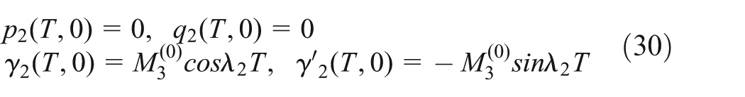
are satisfied. The solutions of equalities (24) have series form of powers of $ϵ$ for $m_1,m_2$ , and $m_4$ and vanish when $ϵ$ tends to zero ( $m_3$ can be considered equal to zero). Under the present circumstances, the periodicity conditions become

$$\begin{array}{c}{m}_1(\cos {\lambda }_1{T}_0-1)+m_2\sin {\lambda }_1{T}_0+ϵC_1^{(1)}(T_0)+\cdots =0\hfill \\ \multicolumn{1}{c}{-m_1\sin {\lambda }_1{T}_0+m_2(\cos {\lambda }_1{T}_0-1)+ϵC_2^{(1)}(T_0)+\cdots =0}\\ \multicolumn{1}{c}{C_4^{(1)}(T_0)+\cdots =0}\end{array}$$

(29)

Taking into account (28), the periodic solutions $p_2(T,ϵ),q_2(T,ϵ),{\gamma }_2(T,ϵ)$ , and $\gamma {\prime }_2(T,ϵ)$ at $ϵ=0$ become

$$\begin{array}{c}{p}_2(T,0)=0,q_2(T,0)=0\hfill \\ \multicolumn{1}{c}{{\gamma }_2(T,0)=M_3^{(0)}\cos {\lambda }_{2}T,{\gamma \prime }_2(T,0)=-M_3^{(0)}\sin {\lambda }_{2}T}\end{array}$$

(30)

with the frequency ${\lambda }_2$ .

Making use of the second integral in (5) and conditions (14), we get

$$\begin{array}{l}{M}_3^{(0)}=\frac{1}{2}{N}_1^{-1}\left[-N_2\pm \sqrt{N_2^2+4N_1{N}_3}\right];\\ N_1\ne 0,N_2^2+4N_1{N}_3>0\end{array}$$

(31)

where $(N_j;j=1,2,3)$ are functions of $h,\beta ,p_{20},q_{20},{\gamma }_{20}$ , and $\gamma {\prime }_{20}$ that can be obtained easily.

On the use of equations (28) and (29), we obtain directly $m_1$ and $m_2$ . The calculations for $m_4$ reveal that it is of the order $O({ϵ}^2)$ .

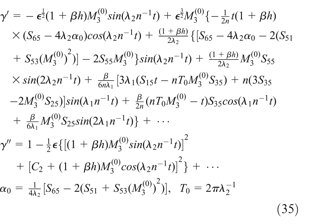
Making use of (8), (13), (19)–(22), and (28), one obtains

$$\begin{array}{c}p={ϵ}^{\frac{1}{2}}{n}^{-1}[C_1+{\mathrm{hM}}_3^{(0)}\cos ({\lambda }_2{n}^{-1}t)]+{ϵ}^{\frac{3}{2}}{n}^{-1}\{\frac{h}{2{\lambda }_2}[2(S_{61}+S_{63})\hfill \\ \multicolumn{1}{c}{-S_{55}{(M_3^{(0)})}^2]+\frac{1}{2{\lambda }_1}[2S_{31}+(2S_{33}-S_{25}){(M_3^{(0)})}^2]-\frac{h}{6{\lambda }_2}\{3[2S_{61}}\\ \multicolumn{1}{c}{+(2S_{63}-S_{55}){(M_3^{(0)})}^2]+S_{65}{(M_3^{(0)})}^2\}\cos ({\lambda }_2{n}^{-1}t)-\frac{\mathrm{ht}}{2n}[2(S_{51}}\\ \multicolumn{1}{c}{+S_{55}{(M_3^{(0)})}^2)-S_{65}+2{\lambda }_2{\alpha }_0]M_3^{(0)}\sin ({\lambda }_2{n}^{-1}t)-\frac{1}{2n{\lambda }_1}\{n[2S_{31}}\\ \multicolumn{1}{c}{+(2S_{33}-S_{25}){(M_3^{(0)})}^2]+M_3^{(0)}{\lambda }_1(t{S}_{36}-n{T}_0{M}_3^{(0)}{S}_{35})\}}\\ \multicolumn{1}{c}{\times \cos ({\lambda }_1{n}^{-1}t)+\frac{1}{2}(M_3^{(0)}{T}_0+2)M_3^{(0)}{S}_{35}\sin ({\lambda }_1{n}^{-1}t)+\frac{h}{6{\lambda }_2}}\\ \multicolumn{1}{c}{\times {(M_3^{(0)})}^2{S}_{55}\cos (2{\lambda }_2{n}^{-1}t)+\cdots }\end{array}$$

(32)

$$\begin{array}{c}q=-{ϵ}^{\frac{1}{2}}{n}^{-1}{\mathrm{hM}}_3^{(0)}\sin ({\lambda }_2{n}^{-1}t)+{ϵ}^{\frac{3}{2}}{n}^{-1}{M}_3^{(0)}\{\frac{\mathrm{ht}}{2n{\lambda }_2}[S_{65}-4{\lambda }_2{\alpha }_0\hfill \\ \multicolumn{1}{c}{-2(S_{51}+S_{53}{(M_3^{(0)})}^2)]\cos ({\lambda }_2{n}^{-1}t)+\frac{h}{2{\lambda }_2}\{[S_{65}-4{\lambda }_2{\alpha }_0}\\ \multicolumn{1}{c}{-2(S_{51}+S_{53}{(M_3^{(0)})}^2)]-2S_{55}{M}_3^{(0)}\}\sin ({\lambda }_2{n}^{-1}t)+\frac{h}{2{\lambda }_2}{M}_3^{(0)}}\\ \multicolumn{1}{c}{\times S_{55}\sin (2{\lambda }_2{n}^{-1}t)+\frac{1}{6n{\lambda }_1}[3{\lambda }_1(t{S}_{15}-n{T}_0{M}_3^{(0)}{S}_{35})}\\ \multicolumn{1}{c}{+n(3S_{35}-2S_{25}{M}_3^{(0)})]\sin (2{\lambda }_1{n}^{-1}t)+\frac{1}{2n{\lambda }_2}(n{\lambda }_2{T}_0{M}_3^{(0)}+t)}\\ \multicolumn{1}{c}{\times S_{35}\cos ({\lambda }_1{n}^{-1}t)+\frac{1}{6{\lambda }_1}{S}_{25}{M}_3^{(0)}\sin (2{\lambda }_1{n}^{-1}t)\}+\cdots }\\ \multicolumn{1}{c}{r=\frac{1}{n}{r}_0-\frac{1}{\mathrm{nb}{r}_{10}}ϵM_3^{(0)}\{[(1+\beta h)[C_2(k+1)-1]+h{C}_1]}\\ \multicolumn{1}{c}{\times (\cos ({\lambda }_2{n}^{-1}t)-1)\}+\cdots }\end{array}$$

(33)

$$\begin{array}{c}\gamma ={ϵ}^{\frac{1}{2}}[C_2+(1+\beta h)M_3^{(0)}\cos ({\lambda }_2{n}^{-1}t)]+{ϵ}^{\frac{3}{2}}\{\frac{(1+\beta h)}{2{\lambda }_2}[2S_{61}+(2S_{63}\hfill \\ \multicolumn{1}{c}{-S_{55}){(M_3^{(0)})}^2]+\frac{\beta }{2{\lambda }_1}[2S_{31}+(2S_{33}-S_{25}){(M_3^{(0)})}^2]-\frac{(1+\beta h)}{6{\lambda }_2}}\\ \multicolumn{1}{c}{\times \{3[2S_{61}+(2S_{63}-S_{55}){(M_3^{(0)})}^2]+S_{55}{(M_3^{(0)})}^2\}\cos ({\lambda }_2{n}^{-1}t)}\\ \multicolumn{1}{c}{+\frac{(1+\beta h)}{2n}{M}_3^{(0)}t[S_{65}-2{\lambda }_2{\alpha }_0-2(S_{51}+S_{53}{(M_3^{(0)})}^2)]\sin ({\lambda }_2{n}^{-1}t)}\\ \multicolumn{1}{c}{+\frac{(1+\beta h)}{6{\lambda }_2}{(M_3^{(0)})}^2{S}_{55}\cos (2{\lambda }_2{n}^{-1}t)+\frac{1}{2n{\lambda }_1}\{n{T}_0{\lambda }_1{(M_3^{(0)})}^2{S}_{35}}\\ \multicolumn{1}{c}{-\beta [2n{S}_{31}+n(2S_{33}-S_{25}){(M_3^{(0)})}^2+{\lambda }_1{S}_{36}{M}_3^{(0)}t]\}\cos ({\lambda }_1{n}^{-1}t)}\\ \multicolumn{1}{c}{+\frac{1}{2}\beta (2+M_3^{(0)}{T}_0)M_3^{(0)}{S}_{35}\sin ({\lambda }_1{n}^{-1}t)+\cdots }\end{array}$$

(34)

$$\begin{array}{c}\gamma \prime =-{ϵ}^{\frac{1}{2}}(1+\beta h)M_3^{(0)}\sin ({\lambda }_2{n}^{-1}t)+{ϵ}^{\frac{3}{2}}{M}_3^{(0)}\{-\frac{1}{2n}t(1+\beta h)\hfill \\ \multicolumn{1}{c}{\times (S_{65}-4{\lambda }_2{\alpha }_0)\cos ({\lambda }_2{n}^{-1}t)+\frac{(1+\beta h)}{2{\lambda }_2}\{[S_{65}-4{\lambda }_2{\alpha }_0-2(S_{51}}\\ \multicolumn{1}{c}{+S_{53}{(M_3^{(0)})}^2)]-2S_{55}{M}_3^{(0)}\}\sin ({\lambda }_2{n}^{-1}t)+\frac{(1+\beta h)}{2{\lambda }_2}{M}_3^{(0)}{S}_{55}}\\ \multicolumn{1}{c}{\times \sin (2{\lambda }_2{n}^{-1}t)+\frac{\beta }{6n{\lambda }_1}[3{\lambda }_1(S_{15}t-n{T}_0{M}_3^{(0)}{S}_{35})+n(3S_{35}}\\ \multicolumn{1}{c}{-2M_3^{(0)}{S}_{25})]\sin ({\lambda }_1{n}^{-1}t)+\frac{\beta }{2n}(n{T}_0{M}_3^{(0)}-t)S_{35}\cos ({\lambda }_1{n}^{-1}t)}\\ \multicolumn{1}{c}{+\frac{\beta }{6{\lambda }_1}{M}_3^{(0)}{S}_{25}\sin (2{\lambda }_1{n}^{-1}t)\}+\cdots }\\ \multicolumn{1}{c}{\gamma ″=1-\frac{1}{2}ϵ\{{[(1+\beta h)M_3^{(0)}\sin ({\lambda }_2{n}^{-1}t)]}^2}\\ \multicolumn{1}{c}{+{[C_2+(1+\beta h)M_3^{(0)}\cos ({\lambda }_2{n}^{-1}t)]}^2\}+\cdots }\\ \multicolumn{1}{c}{{\alpha }_0=\frac{1}{4{\lambda }_2}[S_{65}-2(S_{51}+S_{53}{(M_3^{(0)})}^2)],T_0=2\pi {\lambda }_2^{-1}}\end{array}$$

(35)

It is worthwhile to note that, when the attracting center R tends to infinity and $x_G=y_G=0$ , the gyroscopic motion studied by Sansaturio and Vigueras ²⁵ is obtained. Also, when R tends to infinity beside ${\ell }_1={\ell }_3=0$ , the solution given in Elfimov ¹⁸ is obtained. So, our solution is considered as a generalization of some previous works. Therefore, the present results are in a good agreement with the known previous results of Elfimov ¹⁸ and Sansaturio and Vigueras. ²⁵

Geometrical interpretation

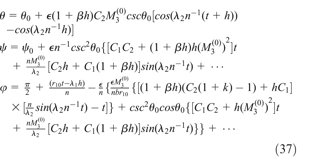
The scope of this section is to investigate the geometrical interpretation of motion in framework of Euler’s angles in terms of $ϵ$ to determine the motion of the gyro at any instant. For this task, the expressions of Euler’s angles $\theta ,\phi$ , and $\psi$ take the following forms ¹¹

$$\begin{array}{l}\theta ={\cos }^{-1}\gamma ″,\stackrel{.}{\psi }=\frac{p\gamma +q\gamma \prime }{1-{\gamma ″}^2},\\ \stackrel{.}{\phi }=r-\stackrel{.}{\psi }cos\theta ,{\phi }_0=ta{n}^{-1}\frac{{\gamma }_0}{\gamma {\prime }_0}\end{array}$$

(36)

where the over dot denotes the derivative with respect to time t. Substituting from the obtained solutions (32–35) into the previous equations (36), we get the Euler’s angles $\theta ,\phi$ , and $\psi$ in the following form

$$\begin{array}{c}\theta ={\theta }_0+ϵ(1+\beta h)C_2{M}_3^{(0)}\csc {\theta }_0[\cos ({\lambda }_2{n}^{-1}(t+h))\hfill \\ \multicolumn{1}{c}{-\cos ({\lambda }_2{n}^{-1}h)]}\\ \multicolumn{1}{c}{\psi ={\psi }_0+ϵn^{-1}\mathrm{cs}{c}^2{\theta }_0\{[C_1{C}_2+(1+\beta h)h{(M_3^{(0)})}^2]t}\\ \multicolumn{1}{c}{+\frac{{\mathrm{nM}}_3^{(0)}}{{\lambda }_2}[C_{2}h+C_1(1+\beta h)]\sin ({\lambda }_2{n}^{-1}t)+\cdots }\\ \multicolumn{1}{c}{\phi =\frac{\pi }{2}+\frac{(r_{10}t-{\lambda }_{1}h)}{n}-\frac{ϵ}{n}\{\frac{ϵM_3^{(0)}}{\mathrm{nb}{r}_{10}}\{[(1+\beta h)(C_2(1+k)-1)+h{C}_1]}\\ \multicolumn{1}{c}{\times [\frac{n}{{\lambda }_2}\sin ({\lambda }_2{n}^{-1}t)-t]\}+\mathrm{cs}{c}^2{\theta }_0\cos {\theta }_0\{[C_1{C}_2+h{(M_3^{(0)})}^2]t}\\ \multicolumn{1}{c}{+\frac{{\mathrm{nM}}_3^{(0)}}{{\lambda }_2}[C_{2}h+C_1(1+\beta h)]\sin ({\lambda }_2{n}^{-1}t)\}\}+\cdots }\end{array}$$

(37)

Consequently, these formulas reveal that the previous attained expressions of Euler’s angles hinge on three arbitrary constants ${\theta }_0,{\psi }_0$ , and $r_0$ .

Simulation and results

The goal of this section is to investigate the graphical representations of the obtained solutions to show the variation of time t on the solutions p and q and to study the stability of these solutions during the motion. So, in order to investigate this purpose, we consider the following data of the gyro

$$\begin{array}{c}A=B=4.5\mathrm{kg}{\mathrm{m}}^2,C=2.3\mathrm{kg}{\mathrm{m}}^2,ϵ=0.1E-03\hfill \\ M=300\mathrm{kg},z_G=0.06\mathrm{m},\lambda =0.7,\hfill \\ p_0=1.67E-05\mathrm{rad}.s^{-1},\hfill \\ q_0=5.23E-08\mathrm{rad}.s^{-1},{\gamma }_0=79.07E-03\mathrm{rad}.s^{-1},\hfill \\ {\gamma \prime }_0=5.44E-03\mathrm{rad}.s^{-1},{\ell \prime }_1=(10,15,20)\mathrm{kg}\mathrm{m}{\mathrm{s}}^{-1}\hfill \\ {\ell \prime }_3=(10,15,20)\mathrm{kg}{\mathrm{m}}^2{\mathrm{s}}^{-1},\hfill \\ R=(600,800,1000)\mathrm{m},g=9.81\mathrm{m}{\mathrm{s}}^{-2}\hfill \end{array}$$

(38)

Figures 2 and 3 show the graphical representations for the attained solution p with time t when the distance between the fixed point O and the attracting center $O_1$ (i.e. R) equals 800 m. In Figure 2, the first component of the gyrostatic moment $\ell {\prime }_1$ equals $(10,15,20)\mathrm{kg}{\mathrm{m}}^2{\mathrm{s}}^{-1}$ and the value of the third component $\ell {\prime }_3$ of the same moment equals $10\mathrm{kg}{\mathrm{m}}^2{\mathrm{s}}^{-1}$ . Conversely in Figure 3, $\ell {\prime }_3$ changes from $10$ to $20\mathrm{kg}{\mathrm{m}}^2{\mathrm{s}}^{-1}$ through the value $15\mathrm{kg}{\mathrm{m}}^2{\mathrm{s}}^{-1}$ and $\ell {\prime }_1=10\mathrm{kg}{\mathrm{m}}^2{\mathrm{s}}^{-1}$ .

Figure 2.

Variation of the solution p via t at $R=800m$ and $\ell {\prime }_3=10\mathrm{kg}{\mathrm{m}}^2{\mathrm{s}}^{-1}$ when $\ell {\prime }_1$ equals $10,15,$ and $20\mathrm{kg}{\mathrm{m}}^2{\mathrm{s}}^{-1}$ .

Figure 3.

Variation of the solution p via t at $R=800\mathrm{m}$ and $\ell {\prime }_1=10\mathrm{kg}{\mathrm{m}}^2{\mathrm{s}}^{-1}$ when $\ell {\prime }_3$ equals $10,15,$ and $20\mathrm{kg}{\mathrm{m}}^2{\mathrm{s}}^{-1}$ .

A conclusion that may be written here is that when $\ell {\prime }_1$ takes the values $(10,15,20)\mathrm{kg}{\mathrm{m}}^2{\mathrm{s}}^{-1}$ (i.e. increases) with the stationary values of R and $\ell {\prime }_3$ , the standing waves with lower frequency are obtained as seen in Figure 2. However, when $\ell {\prime }_1$ becomes stationary besides R with the variation in the values of $\ell {\prime }_3$ , the traveling waves with higher frequency are produced as evident in Figure 3. It is important to note that the amplitudes of the waves increase and the number of oscillations remains unchanged with the increasing $\ell {\prime }_1$ as shown in Figure 2. Moreover, one can observe from Figure 3 that the amplitudes and the number of waves increase with the increasing values of $\ell {\prime }_3$ .

An inspection of Figures 4 and 5 shows the variation of the solution q against time t with the same value of R. In Figure 4, $\ell {\prime }_1$ takes the values $(10,15,20)\mathrm{kg}{\mathrm{m}}^2{\mathrm{s}}^{-1}$ when $\ell {\prime }_3$ becomes constant, that is, equal to $10\mathrm{kg}{\mathrm{m}}^2{\mathrm{s}}^{-1}$ . As indicated in Figure 5, $\ell {\prime }_1$ is equal to $10\mathrm{kg}{\mathrm{m}}^2{\mathrm{s}}^{-1}$ and $\ell {\prime }_3$ takes the values $10,15,$ and $20\mathrm{kg}{\mathrm{m}}^2{\mathrm{s}}^{-1}$ .

Figure 4.

Variation of the solution q via t at $R=800\mathrm{m}$ and $\ell {\prime }_3=10\mathrm{kg}{\mathrm{m}}^2{\mathrm{s}}^{-1}$ when $\ell {\prime }_1$ equals $10,15,$ and $20\mathrm{kg}{\mathrm{m}}^2{\mathrm{s}}^{-1}$ .

Figure 5.

Variation of the solution q via t at $R=800\mathrm{m}$ and $\ell {\prime }_1=10\mathrm{kg}{\mathrm{m}}^2{\mathrm{s}}^{-1}$ when $\ell {\prime }_3$ equals $10,15,$ and $20\mathrm{kg}{\mathrm{m}}^2{\mathrm{s}}^{-1}$ .

When Figure 4 is generally compared with Figure 5 we observe that the amplitudes of the standing waves increase with the increasing values of $\ell {\prime }_1$ (see Figure 4). On the other side, the number of traveling oscillations and the amplitude of the waves increase with the increasing $\ell {\prime }_3$ as seen in Figure 5. This elucidates that the corresponding values of q increases which is in agreement with the increasing p as seen in these figures. In other words, this conclusion can be physically interpreted that there is an increasing of the velocity of the gyro and consequently the kinetic energy increases.

However, when the distance between the fixed point and the attracting center increases, rather different plots are drawn. Figures 6 and 7 represent the influence of increasing R on the solutions p when $\ell {\prime }_1=20,\ell {\prime }_3=10$ and $\ell {\prime }_1=10,\ell {\prime }_3=20$ , respectively. On the other side, Figures 8 and 9 sketch the influence of increasing R on the solutions q when $\ell {\prime }_1=20,\ell {\prime }_3=10$ and $\ell {\prime }_1=10,\ell {\prime }_3=20$ , respectively, with the same considered data of the other parameters in the previous figures.

Figure 6.

Illustration of the variation of the solution p versus t at $\ell {\prime }_1=20\mathrm{kg}{\mathrm{m}}^2{\mathrm{s}}^{-1}$ and $\ell {\prime }_3=10\mathrm{kg}{\mathrm{m}}^2{\mathrm{s}}^{-1}$ when R equals 600, 800, and 1000 m.

Figure 7.

Illustration of the variation of the solution p versus t at $\ell {\prime }_1=10\mathrm{kg}{\mathrm{m}}^2{\mathrm{s}}^{-1}$ and $\ell {\prime }_3=20\mathrm{kg}{\mathrm{m}}^2{\mathrm{s}}^{-1}$ when R equals 600, 800, and 1000 m.

Figure 8.

Illustration of the variation of the solution q versus t at $\ell {\prime }_1=20\mathrm{kg}{\mathrm{m}}^2{\mathrm{s}}^{-1}$ and $\ell {\prime }_3=10{\mathrm{kg\; m}}^2{\mathrm{s}}^{-1}$ when R equals 600, 800, and 1000 m.

Figure 9.

Illustration of the variation of the solution q versus t at $\ell {\prime }_1=10\mathrm{kg}{\mathrm{m}}^2{\mathrm{s}}^{-1}$ and $\ell {\prime }_3=20\mathrm{kg}{\mathrm{m}}^2{\mathrm{s}}^{-1}$ when R equals 600, 800, and 1000 m.

An inspection of (Figures 6 and 8) and (Figures 7 and 9) shows that broadly speaking, when R increases and takes specifically the values 600, 800, and 1000 m, both the standing and progressive waves are obtained through three curves with shorter wavelength and higher frequency. Also, it is clear that both the number of oscillations and the amplitudes of the waves increases with the increasing distance R (see Figures 6 and 8). However, it is not difficult to conclude from Figures 7 and 9 that when R increases, the amplitude of the waves decreases and the number of ripples increases. This indicates the good effectiveness of the gyrostatic moment on the motion. The variation of the solutions between increasing and decreasing gives an indication of increasing or decreasing energy of the gyrostat which can be used in industrial applications.

The most interesting case is to study the phase plane of the obtained solutions through some diagrams. These diagrams have been produced by drawing the solution against its first derivative. Some of these plots with different values of $R,\ell {\prime }_1$ , and $\ell {\prime }_3$ are given in Figures 10 and 11 for the solution p and in Figures 12 and 13 for the solution q. The phase plane plots give an indication about the system is free of chaos.

Figure 10.

The phase plane diagram of the solution p when $R=600m,\ell {\prime }_1=20\mathrm{kg}{\mathrm{m}}^2{\mathrm{s}}^{-1}$ , and $\ell {\prime }_3=10\mathrm{kg}{\mathrm{m}}^2{\mathrm{s}}^{-1}$ .

Figure 11.

The phase plane diagram of the solution p when $R=600m,\ell {\prime }_1=10\mathrm{kg}{\mathrm{m}}^2{\mathrm{s}}^{-1}$ , and $\ell {\prime }_3=20\mathrm{kg}{\mathrm{m}}^2{\mathrm{s}}^{-1}$ .

Figure 12.

The phase plane plot of the solution q when $R=800m,\ell {\prime }_1=20\mathrm{kg}{\mathrm{m}}^2{\mathrm{s}}^{-1}$ , and $\ell {\prime }_3=10\mathrm{kg}{\mathrm{m}}^2{\mathrm{s}}^{-1}$ .

Figure 13.

The phase plane plot of the solution q when $R=800m,\ell {\prime }_1=10\mathrm{kg}{\mathrm{m}}^2{\mathrm{s}}^{-1}$ , and $\ell {\prime }_3=20\mathrm{kg}{\mathrm{m}}^2{\mathrm{s}}^{-1}$ .

Conclusion

A conclusion that may be constructed here is that the small parameter method of Poincaré is applied to obtain the approximate analytic periodic solutions for the mentioned problem up to the fraction order 3/2 of the small parameter $ϵ$ . The obtained results of this article are in good agreement with Elfimov ¹⁸ (for the uniform field case, that is, $N\approx 0$ and $\underset{¯}{\ell }=0$ ) and with Sansaturio and Vigueras ²⁵ when R tends to infinity and $x_G=y_G=0$ . So, our periodic solutions (32–35) can be considered as a generalization of these works. The achieved solutions are anatomized geometrically with the aid of the Euler’s angles to portray the motion at any instant of time. The standing waves with larger wavelength having some nods are produced when the first component of the gyrostatic moment takes different values with the stationary values of other parameters. Moreover, if $\ell {\prime }_3$ takes different values, with the constant values of other parameters, the traveling waves are produced with shorter wavelength besides increasing the amplitude of the waves. Consequently, the energy of the gyro increases, which has a significant impact in industrial applications. This is due to the variation of the gyrostatic moment components, which elucidates the importance of these components. The results also indicate that when the distance R between the fixed point and the attracting center increases, the progressive waves are obtained and the wavelength of these waves decreases. Then, the number of oscillations and the amplitudes increases or decreases leading to increasing or decreasing in the velocity of the gyro and therefore increasing or decreasing in the gyro energy occurred. It reinforces the importance of existence of the Newtonian force field and the change in the distance R. The good effects of the two components of the gyrostatic moment vector and the Newtonian force field, on the considered problem are obvious from the graphical representation. Some phase plane diagrams are plotted for the attained solutions.