A computational study on gas–liquid flow in a lime slurry pond equipped with a rotary jet mixing system

Abstract

The flue-gas desulfurization model was studied through computational fluid dynamics software. The oxidation air was asymmetrically pumped into the slurry pond. A rotary jet mixing system was established at the bottom center of the pond to agitate the lime slurry. The Navier–Stokes equation as the control equation, the standard k–ε turbulence model, sliding grids structure, and three-dimensional Eulerian multiphase flow of lime slurry were used for the numerical simulation. The independence of the meshes and the time step was verified. The distribution of the concentration of oxidation air and influents on the velocity of flow was analyzed with five angular velocities (0.01, 0.10, 0.20, 0.50, and 1 rad/s) for the rotary jet mixing. The simulation results showed that the angular velocity has a great influence on the velocity of the slurry and the distribution of the oxidation air.

Introduction

The technology of wet desulfurization is the mainstream in the coal-fired power plant desulfurization treatment in China. ¹ Limestone-gypsum technology uses limestone or lime slurry as the absorbent, SO₂ in the flue gas, CaCO₃ in the slurry, and the pumped air all take part in oxidation reaction. The product recycles in the form of gypsum. In this process, the oxidation reaction occurs in the absorption tower, which need to have mixing facilities installed to ensure that the reactant fully reacts. The jet mixer has been widely used in solid–liquid suspensions, liquid mixing reactions, gas–liquid mass transfer, and other fields. It is believed that it can be used in the wet desulfurization system.

In recent years, the study of the rotary jet mixing (RJM) system has achieved some results. Maruyama et al. ² and Yianneskis ³ found that the mixing time is related to the depth of the liquid, the height, and the angle of the nozzle. Grenville et al.^4,5 found that the mixing time is determined by the energy dissipation rate of the flow field away from the nozzle. YL Tian et al. ⁶ studied a high viscosity fluid, using the standard k–ε turbulence model to do a full three-dimensional (3D) flow field numerical simulation, estimating the process of the jet and mixing effect. Wei ⁷ studied the hydraulic characteristics of a power turbine for a large-scale industrial oil tank, using the computational fluid dynamics (CFD) technique to simulate the RJM jet flow of the hybrid system. HH Li et al. ⁸ introduced the working principle of a rotary jet stirring mixer and analyzed its economic benefit. XP Wang^9,10 studied the flow field and the velocity attenuation regularity of a jet with different nozzle diameters, different jet velocities, and different tank sizes. SY Chen et al., ¹¹ JJ Mao ¹² , and FC Xie ¹³ simulated the flow field changes of the five-layer distribution of gasoline components in the RJM system using CFD software, and explored the regularity of the mixing time at different nozzle angles and different rotational angular velocities.

Under different angular velocity of the RJM system, this study simulates the effect on the distribution of oxidation air influenced by the nozzle inlet velocity with the jet mixing. The inherent mixing law and dynamic characteristics will provide a useful basis for the application of the RJM system in the flue absorption process of wet limestone slurry pond.

Gas–liquid mixed 3D model

Control equations

In this study, the heat transfer and temperature variation in the flow field were neglected. The turbulence under jet mixing is very complicated. The 3D Navier–Stokes (N-S) equation and standard k–ε equations were used as the control equations.

Continuous equation

$$\frac{\partial u_i}{\partial x_i}=0$$

(1)

Momentum equation

$$\rho \frac{\partial u_i}{\partial t}+\rho u_j\frac{\partial u_i}{\partial x_j}=\rho f_i-\frac{\partial p}{\partial x_i}+\frac{\partial }{\partial x_{\mathrm{i}}}\left[{\mu }_{\mathrm{eff}}(\frac{\partial u_i}{\partial x_j}+\frac{\partial u_j}{\partial x_i})\right]$$

(2)

k–ε equations

$$\begin{array}{l}\rho \frac{\partial k}{\partial t}+\rho u_j\frac{\partial k}{\partial x_j}=\frac{\partial }{\partial x_j}\left[\left(\mu +\frac{{\mu }_t}{{\sigma }_k}\right)\frac{\partial k}{\partial x_j}\right]+P_k-\rho \epsilon \\ \rho \frac{\partial \epsilon }{\partial t}+\rho u_j\frac{\partial \epsilon }{\partial x_j}=\frac{\partial }{\partial x_j}\left[\left(\mu +\frac{{\mu }_t}{{\sigma }_{\epsilon }}\frac{\partial \epsilon }{\partial x_j}\right)\right]+\frac{\epsilon }{k}(C_{1\epsilon }{P}_k-C_{2\epsilon }\rho \epsilon )\end{array}$$

(3)

where u_i and u_j are velocity tensors; x_i and x_j are displacement tensors; ρ is the density; t is the time; µ is the kinetic viscosity; k is the turbulence kinetic energy; and ε is the turbulence dissipation rate

$$\begin{array}{c}{\mu }_{\mathrm{eff}}-\mathrm{effective\; viscosity},{\mu }_{\mathrm{eff}}=\mu +{\mu }_t;\hfill \\ {\mu }_t-\mathrm{turbulent\; viscosity},{\mu }_t=P{C}_{\mu }\frac{k^2}{\epsilon };\hfill \\ f_i-\mathrm{unit\; mass\; force};P_k={\mu }_t[\frac{\partial u_i}{\partial x_j}+\frac{\partial u_j}{\partial x_i}]\left(\frac{\partial u_i}{\partial x_j}\right)\hfill \end{array}$$

Using the symmetric model as the drag model

$$K_{\mathrm{pq}}=\frac{{\alpha }_p({\alpha }_p{\rho }_p+{\alpha }_q{\rho }_q)f}{{\tau }_{\mathrm{pq}}}$$

(4)

$$f=\frac{C_D\mathrm{Re}}{24}$$

(5)

$${\tau }_{\mathrm{pq}}=\frac{({\alpha }_p{\rho }_p+{\alpha }_q{\rho }_q)\left(\frac{d_p+d_q}{2}\right)}{18({\alpha }_p{\mu }_p+{\alpha }_q{\mu }_q)}$$

(6)

$$C_D=\{\begin{array}{cc}24(1+0.15{\mathrm{Re}}^{0.0687})/\mathrm{Re}\hfill & \mathrm{Re}\le 1000\hfill \\ \multicolumn{1}{c}{0.44}& \mathrm{Re}>1000\hfill \end{array}$$

(7)

where C_D is the drag coefficient, K_pq is the interphase exchange coefficient, and Re denotes Reynolds number.

Physical model

The height of the lime slurry pond was 15.540 m and the pond radius was 8.200 m as shown in Figure 1. Four non-uniform air inlets and five groups of rotary jet mixers were installed in the lime slurry pond. The six nozzles were uniformly distributed around the rotary stirrer. As shown in Figure 2, a pair of nozzles was horizontally arranged. The remaining two pairs of nozzles had the same downward inclined angle 60° with the horizontal surface. The nozzle diameter was 0.2 m. The distribution of the air inlet and the RJM is shown in Figure 3. Fluid entered the stationary fluid at a certain speed perpendicular to the exit cross section, forming a submerged jet. The calculation area was the external flow field of the jet mixer. The FLUENT group of ANSYS14.0 was selected to establish the model of the lime slurry pond. The 3D model of the flow field was established by Gambit. In this study, five kinds of working conditions of the same physical model were compared. The parameters are shown in Table 1.

Figure 1.

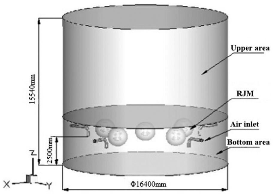
Physical model of the slurry pond.

Figure 2.

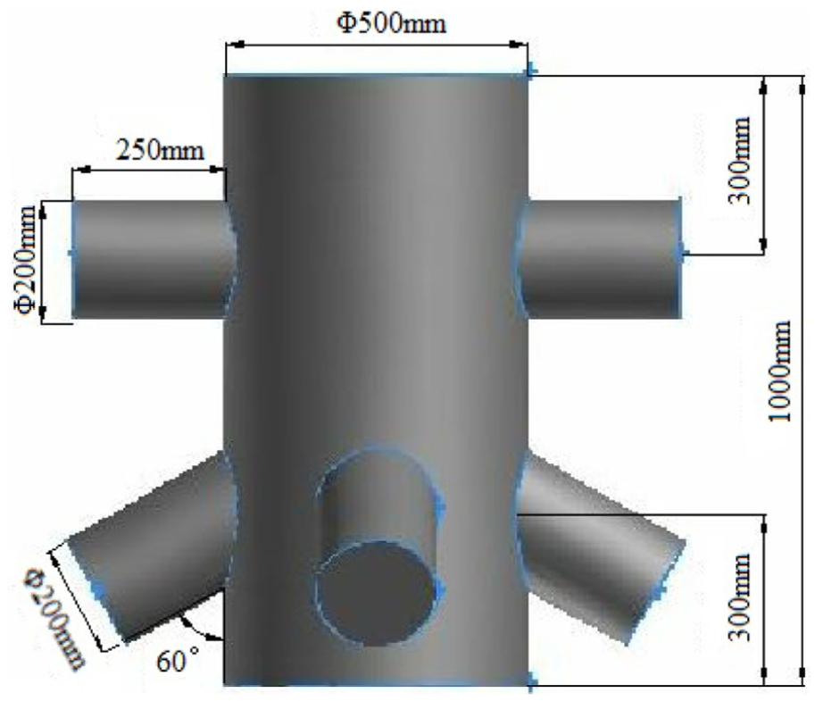
Rotating jet mixer.

Figure 3.

Rotary jet distribution.

Table 1.

Simulation conditions.

Conditions	Parameters
R1	V = 50 m/s, ω = 0.01 rad/s
R2	V = 50 m/s, ω = 0.10 rad/s
R3	V = 50 m/s, ω = 0.20 rad/s
R4	V = 50 m/s, ω = 0.50 rad/s
R5	V = 50 m/s, ω = 1.00 rad/s

V: inlet velocity of the liquid phase; ω: rotation angle velocity.

Meshing and boundary conditions

The simulation used standard air and water as the working fluid. The block partition method was used to divide the flow field because the volume of the model was too large. As shown in Figure 4, the grid was divided using Cooper in the upper part of the pond and the inlet of the air. The type of the grid was a regular hexahedron. At the bottom of the pond and the RJM, the grid was divided by the way of the Tet/Hybrid and the type of the grid was a tetrahedron/hybrid grid.

Figure 4.

Grid distribution of the slurry pool model.

The entrance of the gas and liquid phase was defined as mass flow inlet and velocity inlet, respectively. The export of the model was defined as the pressure outlet, and the pressure was 101325 Pa. The interface between the model block was defined as the INTERFACE. The rest of the wall was defined as the WALL.

The numerical simulation started without air in the pond to obtain the liquid phase flow field. The air entrance was opened when the liquid flow field was stable. The amount of air gradually increased after a small amount of air had entered the lime slurry pond. The air was set to 3 mm discrete bubbles. The finite volume method was used for calculations. The modified quick delay differential discrete technique was used for the liquid phase and the upwind difference scheme was used for the diffusion phase. Pressure velocity coupling was solved using the SIMPLE method. The momentum, kinetic energy, and dissipation rate were solved by the second-order upwind scheme.

Grid independence and time step independent verification

Grid independence verification

The model time step was 0.05 s, the outlet velocity of the RJM was 50 m/s, and the rotational angular velocity was 0.2 rad/s. The total number of grids is shown in Table 2. The optimum number of grids was determined by the volume of fraction (VOF) distribution of the area at Z = 2 m and Z = 10 m that were compared with each other.

Table 2.

The grid number statistics.

No.	Air inlet pipe	RJM	The upper pool	The lower pool	Number of grids
	Cooper	T-grid	Cooper	T-grid
1	10,080	45,097	383,625	891,592	1,330,394
2	10,080	45,097	383,625	2,200,052	2,638,854
3	10,080	45,097	550,126	2,471,683	3,076,986

RJM: rotary jet mixing.

The result shows that when the number of grids was 1.33 × 10⁶, the distribution of oxidized air at Z = 2 m and Z = 10 m was much smaller than the other two groups. When the grid number increased from 2.64 × 10⁶ to 3.08 × 10⁶, the distribution of oxidized air and the region of high concentration at Z = 2 m were similar to that at Z = 10 m. Considering the simulation time, the 2.64 × 10⁶ grid was selected.

Time step independent verification

As defined above, the number of the grid was 2.64 million for the time step independent verification. The outlet velocity of the RJM was 50 m/s, and the rotational angular velocity was 0.2 rad/s. The time step was chosen as 0.05, 0.1, and 0.2 s, respectively. The optimum time step was determined by the VOF nephogram of the area at Z = 2 m and Z = 10 m that were compared with each other.

The result showed that the distribution of oxidation air was very uniform when the time step was 0.05 and 0.1 s in an area of Z = 2 m. A low concentration region appeared along the wall of the lime slurry pond when the time step was increased to 0.2 s. When the time step was 0.2 s, at the area of Z = 10 m, the distribution of oxidation air was different from the other two groups. Overall, the distribution of oxidation air was similar. When the time step was 0.05 and 0.1 s, the concentrations were similar. But when it increased to 0.2 s, an obvious difference appeared. Thus, 0.1 s was selected as the time step.

Results and discussion

In the simulation, the rotational angular velocity of the RJM had an obvious effect on the gas–liquid flow field of the lime slurry pond, so it was chosen as the variable for study.

When the outlet velocity of the RJM was 50 m/s, the upper part of the lime slurry pond was stable and it was not directly impacted by the jet. The flow field was extremely complicated at the bottom of the pond because of the direct impact by the jet. The result was analyzed from the oxidation air distribution and velocity field as follows.

The influence of the rotational angular velocity on the distribution of oxidation air

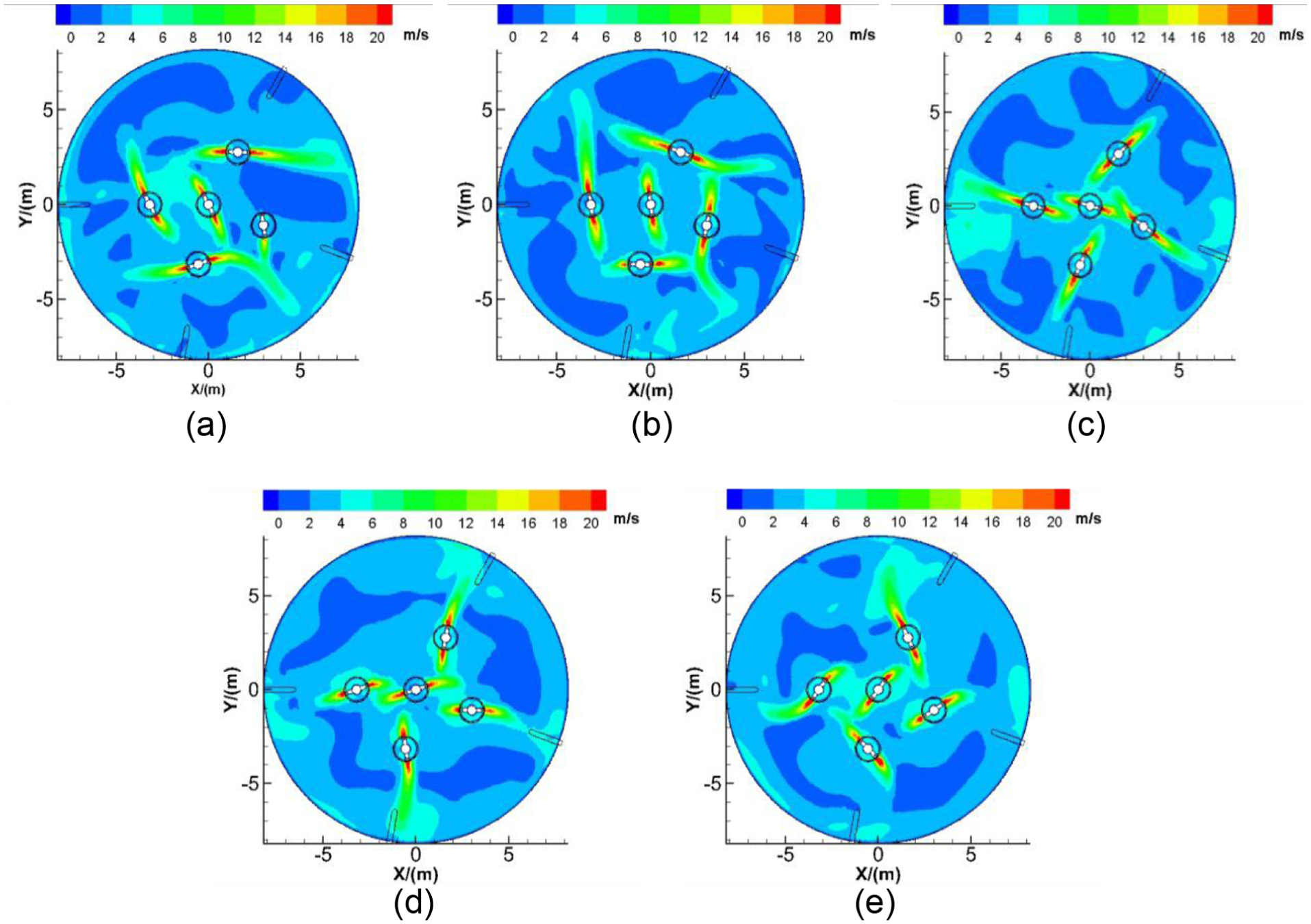
As shown in Figure 5, with an increase in the rotational angular velocity of the RJM, the distribution of the oxidation air tended to be uniform at first and then deteriorated. Under the condition of R2 (0.1 rad/s) and R3 (0.2 rad/s), the oxidation air could cover most of the area of the pond and the concentration gradient was small.

Figure 5.

Distribution nephogram of oxidation air in the lime slurry pond: (a) R1 (ω = 0.01 rad/s), (b) R2 (ω = 0.10 rad/s), (c) R3 (ω = 0.20 rad/s), (d) R4 (ω = 0.50 rad/s), and (e) R5 (ω = 1.00 rad/s).

For the operation of R4 (0.5 rad/s) and R5 (1.0 rad/s), the influence range controlled by the air distribution peak is about 1.5 m along the Z-direction, but the air VOF rapidly reduced to 0.02–0.03 or so from the height of 5 m. In the area around the air entrance, the inlet air gathered to perform VOF peak at the level of the rotary jet installation.

Under the condition of R1 (0.01 rad/s), R4 (0.50 rad/s), and R5 (1.00 rad/s), the oxidation air was gathered in a small area which could affect the oxidation results.

After introducing the RJM, the central portion of the pond became the weak link because there was no inlet of oxidation air which is proved in Figure 5. As is shown in Figure 6, the VOF of the oxidation air was stable at about 0.02 and the fluctuation was very small in the center of the upper part of the pond at R2 condition which was better than the other four conditions.

Figure 6.

Distribution of oxidation air in the center of the pond.

Overall, with the increase in the angular velocity, the distribution of the oxidation air tended to be uniform at first and then deteriorated. The R2 condition was better than the other conditions both in the distribution and the gradient variation of the oxidation air.

The influence of the rotational angular velocity on the velocity field

The influence of the rotational angular velocity on the jet length

The rotational angular velocity of RJM has a great influence on the velocity field of the lime slurry pond. The most intuitive performance is the change of the jet length.

Under all the five conditions, it is easy to see that the submerged jet core section was not evidently influenced by the angular velocity. But, the jet boundary layer gradually reduced because of the tangential velocity getting higher in the jet body section.

The developing trend of the body section was destructed by the entrainment effect under the constant surrounding pressure, the jet length of R2 condition decayed after it reached the maximum value. With an increase in the angular velocity, the jet length tended to increase at first and then to decrease as shown in Figure 7.

Figure 7.

Jet velocity nephogram of horizontal nozzle (Z = 3.915 m) of RJM: (a) R1 (ω = 0.01 rad/s), (b) R2 (ω = 0.10 rad/s), (c) R3 (ω = 0.20 rad/s), (d) R4 (ω = 0.50 rad/s), and (e) R5 (ω = 1.00 rad/s).

The jet length directly affected the dispersion result. The reach of the jet was greater at low angular velocity (R2 condition) than that at high velocity (R5 condition). This is why the distribution of oxidation air in R2 was superior to R5.

The influence of the rotational angular velocity on the lateral velocity

The lateral velocity near the outlet of the oxidation air (L-1 in Figure 8) had a great influence on the distribution of the oxidation air. The distributed velocity whose value was equal to the square root of sum of square of direction speed along X and Y was introduced. As shown in Figure 9, the maximum distributed velocity of oxidation air was located at a height of about Z = 2–5 m, which was in line with the RJM. With the increase in the rotational angular velocity, the distributed velocity of the oxidation air increased and then decreased. It can easily be seen that the velocity was the same as the distributed velocity of oxidation air in R2 condition which also indicates that the oxidation was well distributed. It also shows that the difference between the velocity and the distributed velocity in R1 condition was smaller than that in R5 condition. This is because the velocity magnitude in Z-direction for R1 was a little higher than two other states to restrict the air fully distributed. Along the pond height, the average velocity difference is 1.1 m/s for R1 and 2.25 m/s for R5, respectively.

Figure 8.

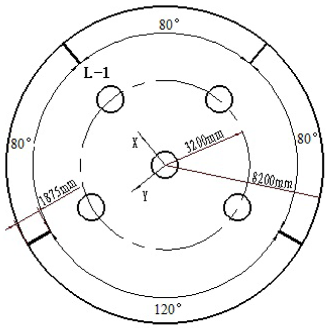
L-1 in the lime slurry pond.

Figure 9.

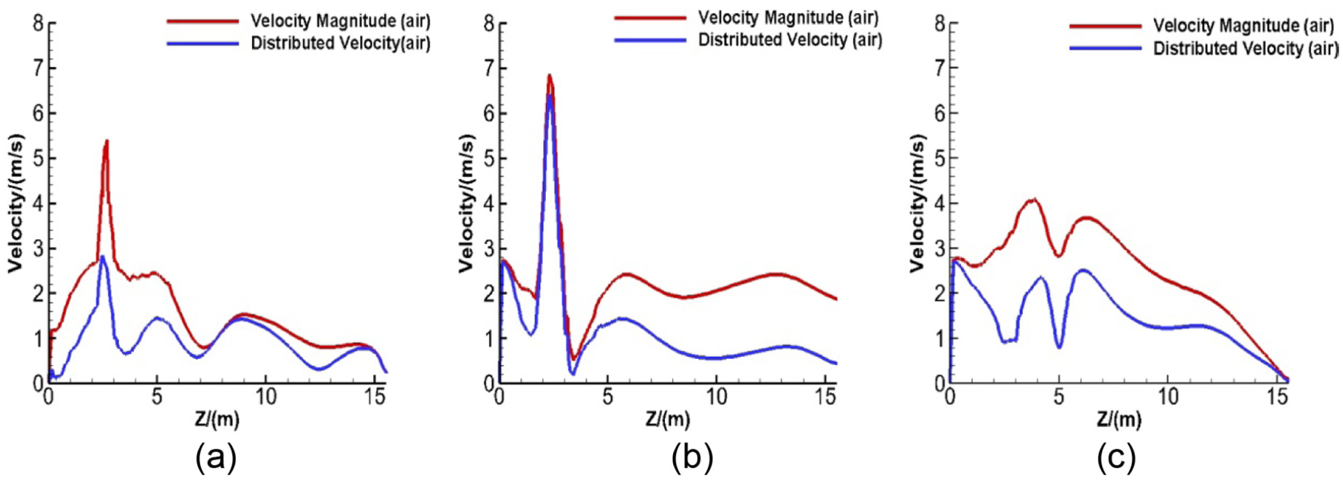
Velocity of oxidation air at L-1 of the lime slurry pond: (a) R1 (ω = 0.01 rad/s), (b) R2 (ω = 0.10 rad/s), and (c) R5 (ω = 1.00 rad/s).

For R5 condition, due to the shortening of the jet length, the radial velocity turns to be low, the air velocity in the Z-direction is increased, and the lateral velocity peak value is lower than the condition of R1 and R2.

The influence of the rotational angular velocity on the velocity of height Z

As a whole, the integral shape of the fluid can be inferred from the velocity at Z-direction. As shown in Figure 10, the slurry moved at a high speed close to the wall of the pond upward to the top and then gathered in the middle. The circulation was restarted with the slurry moving downward along −Z.

Figure 10.

Velocity nephogram of the Z-direction: (a) R1 (ω = 0.01 rad/s), (b) R2 (ω = 0.10 rad/s), and (c) R5 (ω = 1.00 rad/s).

With an increase in the rotation angular velocity, the area affected by the rising fluid was increased. This is because the lateral dispersion of the fluid near the wall was insufficient. The oxidation air was gathered with the rising fluid near the wall, so the concentration near the wall was higher than other areas, which is consistent with the result shown in Figure 5.

With an increase in the rotational angular velocity, the velocity of −Z first increased and then decreased, and the difference of the velocity between the oxidation air and slurry was reduced at the bottom of the pond under all three conditions as shown in Figure 11. This is because of the turbulence intensity getting gradually lower from 0.021 to 0.001 from the bottom to the free surface. In the middle of the pond, the velocity of Z in the oxidation air was about 0.4 m/s less than that in the slurry and showed the same tendency. The oxidation air was transported by the slurry under this condition. In the upper of the pond, the velocity in the oxidation air and in the slurry was both increased along the direction of −Z from the free surface. This shows that the overall velocity of the lime slurry pond slightly increased with the increase in the rotational angular velocity.

Figure 11.

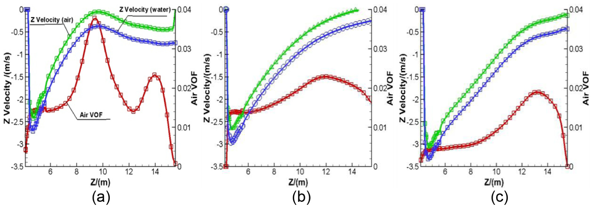
Distribution of velocity at the Z-direction in the center of the lime slurry pond: (a) R1 (ω = 0.01 rad/s), (b) R2 (ω = 0.10 rad/s), and (c) R5 (ω = 1.00 rad/s).

In the slurry bottom, the maximum velocity in the negative Z-direction increased first and then decreased under R1, this is accord with the air lateral velocity distribution. For R1, the velocity difference between air and slurry got evidently higher than R2 and R5 which is due to the high turbulent intensity in the pond. The difference led to the intensive movement in the Z-direction, but the air dispersion was suppressed from the height of 10 to 12 m, the slurry push the air up forward dispersion with the kinetic energy difference until 14 m and then decreased to the free surface. So, the air VOF showed two peak distributions in the whole view. The most intensive dispersing area was located at the tank height of 2–5 m where the rotary jet was equipped.

Conclusion

The following conclusions are drawn from numerical simulation:

1. With an increase in the rotation angular velocity, the slurry mixing area agitated by the jet is decreased, but the vertical velocity of the slurry increased.

2. The distribution of the oxidation air tends at first to be uniform and then to deteriorate with an increase in the rotational angular velocity. The most uniform state can be reached at 0.10 rad/s.

3. The distribution of lateral velocity of the oxidation air has the same tendency as the oxidation of air concentration. It can be seen that the distribution of the oxidation air is mainly controlled by its lateral velocity.