
Abstract
SO2 emissions are known to pose great harm to both human health and atmospheric air, and flue gas generated from coal-fueled power plant is the prime source of sulfur dioxide. For this reason, flue gas desulfurization (FGD) technology has found wide applications in most coal-fired power stations. Correctly describe the dynamic behavior of an FGD process is the precondition of controlling it effectively. However, FGD process modeling is by no means an easy task, as the underlying process dynamics are highly nonlinear in nature, meanwhile time-delay effect is significant therein. Long short-term memory (LSTM) network possesses remarkable long-term memory capability, hence it is anticipated to have a powerful identification capability. In this paper, the connection between deep learning and system identification is established, further a unidirectional/bidirectional LSTM deep network is designed and employed to identify a real FGD process. Simulation results clearly demonstrate the effectiveness of deep learning-based identification approach, and the superiority of deep LSTMs over other conventional identification models is also verified.
Keywords
Introduction
It is the fact that a large amount of sulfur dioxide (SO2) is produced during the coal combustion process, which poses a great threat to both ecological environment and human health. For this reason, the SO2 emission standard for coal-fired power stations in China is gradually becoming tighter in recent years, which states the SO2 emission is not allowed to excess 35 mg/Nm3. 1 For most thermal power plants, FGD installations must be equipped for SO2 removal purposes. Among various FGD techniques, limestone-based flue gas desulfurization (LFGD) technique is the most mature one and has been extensively applied in power plants. For the satisfactory control of outlet SO2 concentration, FGD process dynamics must be adequately captured. In fact FGD modeling is a formidable problem, as the process has highly nonlinear dynamics while existing large time delay. Over the past few decades, there have been considerable numbers of studies in the area of FGD process modeling. Concerning mechanistic models, the heat and mass transfer theory is widely employed to describe an FGD process, the reader is referred to some representative works (e.g. Gage and Rochelle, 2 Brogren and Karlsson, 3 and Eden and Luckas 4 ) for more details. In recent years, there has also been a great deal of research activity in this direction. In Wang et al., 5 a mechanistic model was developed for a micro vortex flow scrubber based on heat and mass transfer characteristics therein, experimental results show validity of the proposed model under varying operating conditions. An analysis model that for the first time combines reaction kinetics and physical mass transfer theory was proposed in Zhang et al., 6 with which characteristics of bubble formation in liquid stage can be determined accurately. 7 focuses on SO2 absorption process in the desulfurization tower, and a comprehensive model that combines transfer process with chemical reactions through Eulerian-Lagrangian method was suggested, and it was shown that the model was able to improve the SO2 removal efficiency for a 330 MW commercial-scale power unit. Due to space limitation interested readers are referred to Flagiello et al., 8 Zhao et al., 9 and Cui et al. 10 for other first principle based modeling approaches. Given the high-level complexity of FGD process, identify an FGD process using merely input-output observations is not a trivial task. As a consequence, the black-box modeling is less frequently used for the FGD process modeling task as compared to mechanistic models. A regression model is established in Hou et al. 11 with the use of operating data of an FGD system, then the multi-objective programing is performed to find optimal parameters such that the system can operate both safely and economically. The universal approximation capability of neural networks makes it a prime candidate to perform the identification task of FGD process. A hybrid model is designed in Guo et al. 12 to provide a prediction for outlet SO2 concentration of a 1000-MW coal-fired unit. The model contains a mechanism model and a multi-input network, simulation results show its effectiveness as compared to classical neural models. In Villanueva Perales et al., 13 the nonlinearity in FGD process is described by a static neural model, based on which a predictive controller is designed to regulate the slurry pH. A BP neural network optimized by the genetic algorithm is applied in Ren et al. 14 to model the FGD process, and both SO2 removal efficiency and operating performance are improved with the proposed model. As for other FGD modeling approaches concerning neural network, the reader is referred to Yang et al. 15 and Liu et al. 16 Owing to the complexity of chemical reaction in an FGD process, the focus in this research is on data-driven identification approach. It is interesting to note that the feedforward network is chosen as an FGD model in most works mentioned above, whereas the time sequential information incorporated in input-output observations cannot be captured by a static architecture. The highly nonlinear dynamics in FGD process calls for some cutting-edge techniques to further improve the identification performance. To fill this gap, DL is integrated into the SI field and applied to identify the FGD process, to the best of our knowledge, none of the earlier works ever attempted in this field. This study makes several significant technical contributions. Firstly, a unidirectional/bidirectional LSTM deep network are designed, and used for the first time successfully in a flue gas desulfurization process identification problem, and shows outstanding identification performance, which provides a promising solution for learning dynamics in an FGD process. Secondly, the connection between non-linear dynamic system identification and deep learning approach is established and verified through the case study of FGD. Finally, in a broader sense, the proposed LSTMs deep learning model can enrich the model selection in the system identification field, which are applicable to different process identification scenarios.
In the remainder of the paper, the FGD process is briefly described and the identification problem is formulated mathematically in next section. Thereafter, in Section 3, the relationship between DL and system identification is first provided, then the applicability of using deep learning to identify non-linear dynamics is analyzed theoretically. Section 4 contains the detailed information of LSTM-based dynamic model. Simulation studies are given in Section 5 and finally relevant conclusions are drawn in Section 6.
FGD principles and problem formulation
Aiming at familiarizing the reader with the FGD process and the identification problem under study, this section first deals with a brief overview of the FGD system, after that the identification problem concerning FGD process is discussed.
Principles of flue gas desulfurization
The installation of FGD units has the purpose of removing SO2 emissions from large-scale electric utility boilers. According to Córdoba 17 and Kumar and Jana 18 with limestone chosen as the absorbent, available FGD techniques can be divided into three categories according to status of limestone, they are: limestone-based dry/semi-dry/wet FGD. Among above approaches, the wet limestone FGD is the most extensively used technique due to its superior desulfurization performance and high reliability. The underlying principle of FGD lies in the interaction between SO2 contained in flue gas and limestone slurry, by sparging air into the reaction tank, gypsum is produced and the overall reaction is
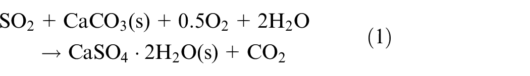
The whole procedure of LFGD process is depicted in Figure 1, we broadly classify the desulfurization process into three parts. The first part is the absorbent slurry preparation, where finely ground limestone slurry is produced and pumped to the storage tank. The second part is the core of the FGD process which serves to eliminate SO2 in the flue gas, and the whole desulfurization process takes place in a spray tower. As shown in Figure 1, the untreated flue gas is fed into the spray tower from the bottom, on the other hand, the reagent slurry is pumped from the reaction tank to spray headers. In such a case, the flue gas is brought into countercurrent contact with the limestone reagent, and SO2 absorption thus takes place. Finally the desulfurized flue gas is passed through mist eliminators followed by discharging into the air. The last part in FGD concerns gypsum dewatering, to be specific, the gypsum slurry filtrate is dewatered through hydrocyclone and the gypsum (
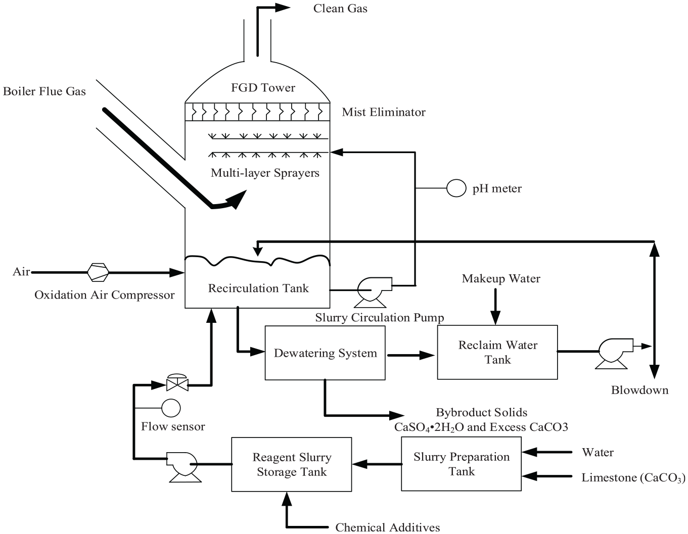
A schematic illustration of FGD process.
Problem formulation
In most cases, chemical processes exhibit non-linear and non-stationary behavior, and the FGD process under study is not an exception. The distinct nonlinearity in FGD process stems from dynamics in thermodynamic relations, chemical reactions, etc. Furthermore, a high time delay often exists in industrial processes, which makes FGD modeling really a challenging problem in the field of system identification. Considering the complicated chemistry concerned in the desulfurization process, the data-driven based modeling approach is more practically reasonable. Assuming the FGD process to be identified is governed by the following vector difference equation
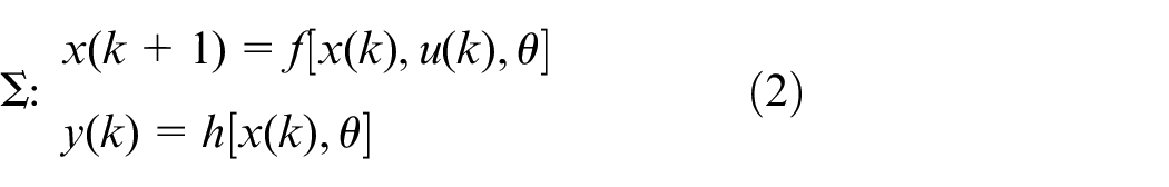
where the input
Let
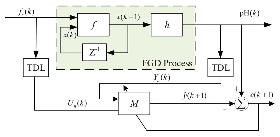
Schematic description of FGD process identification system. The shaded region represents FGD process in form of equation (2), f s (k) and pH(k) denote feeding flow of slurry and slurry pH value at instant k, respectively.
Deep learning and nonlinear dynamic system identification
In this section, the relationship between DL and system identification will be discussed, this will set the stage for applying deep learning techniques to FGD process modeling problem.
Description of neural network and deep neural network
Basically, a neural network (NN) is an architecture that is comprised of a number of interconnected elementary units called neurons. The term “neuron” refers to an operator that maps
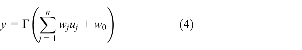
where
where
Nonlinear system identification and network implementation
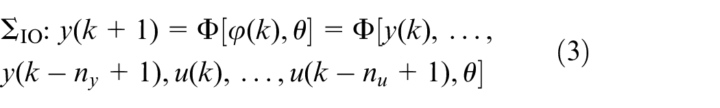
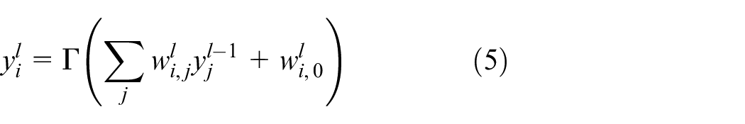
SI is a well-developed field in the control community, there have been an abundance of publications in this area (e.g. Prochazka et al. 22 and Juang 23 ). Nonlinear system identification is a more challenging problem as compared to its linear counterpart. Despite the realization of f and h in (2) involves multiple choices, the neural network, as a universal approximator, 24 is typically the most favored method for this purpose. The feedforward network could be represented as
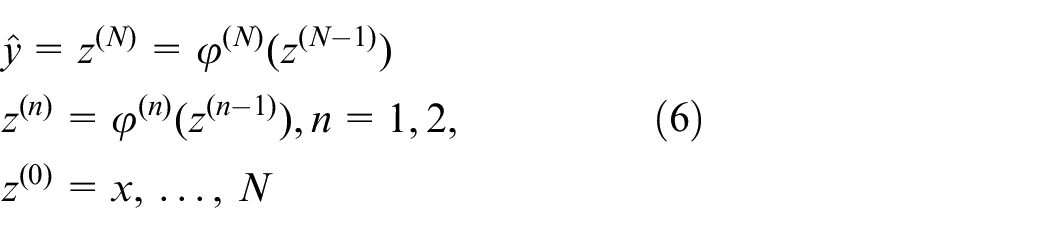
where x, z(n),
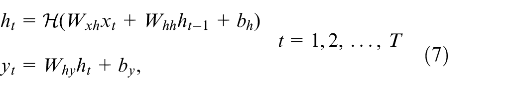
where
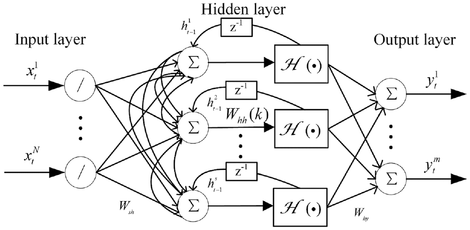
Schematic architecture of the recurrent multilayer perceptron. z−1: one time lag.
The nonlinear mapping defined by (5) more closely matches the true system (2) in format, thus theoretically has advantages over the NARX network in system modeling.
Deep learning based nonlinear system identification
For modeling process with highly nonlinear dynamics, such as the FGD process studied in our paper, neither shallow RNN or NARX network is a good choice due to their structural limitations. It is for such cases that more advanced approaches are called for. The field of DL has gained considerable attention over the past few years, and DL techniques are now applied in wide spans of areas (such as text classification,
25
visual recognition,
26
etc.). Among many branches of DL, the most relevant one for system identification is temporal-sequence learning (TSL), and deep RNN, as the most frequently used TSL model, can also be applied in the system identification field. The word “deep” in deep learning means multiple layers (e.g. convolutional layer, recurrent layers, etc.) are stacked together to such that extremely complicated non-linear dynamics can be captured. As an example, RNN in (5) is modified to the deep version as below. Denoting the sequence in nth hidden layer by
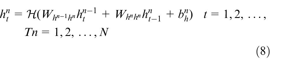
where

LSTMs deep dynamic neural network
This section consists of two parts, the first part deals with a brief overview of LSTMs network; and the use of deep LSTMs for system identification purpose is presented in the second part.
Long short-term memory
LSTM network that was originally introduced in Hochreiter and Schmidhuber 28 is a modified version of standard RNN, where gate units are added to guarantee constant error flow inside the cell and thus can avoid the gradient exploding/vanishing problem. LSTMs are appealing from a system identification viewpoint, due to its superior ability to learn long range dependencies as compared to simple RNNs. 29 An LSTM unit is made up of a cell and three gates (i.e. the input gate, the output gate and the forget gate), wherein the forget gate serves to determine how to preserve cell states in previous time steps, while the input/output gate plays the role of controlling how information is entered and removed from the LSTM unit at each time instant. With the combined effects of gating units, the regulation of information flow is achieved, which in turn enables long-term memory of the LSTM network. For illustrative purposes, the internal and external architecture of an LSTM unit is shown below.
The top plot in Figure 4 shows the inner structure of an LSTM unit, where
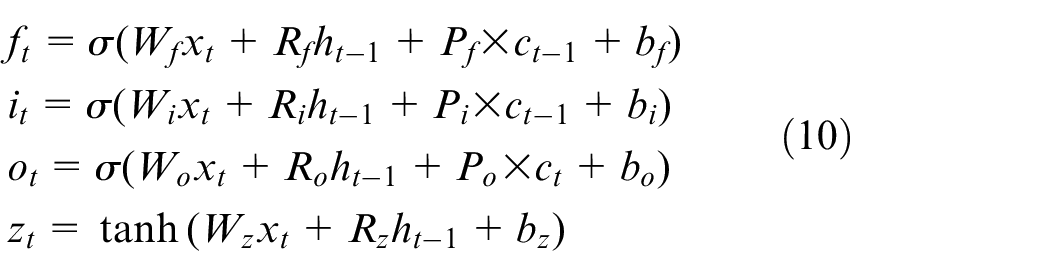
where
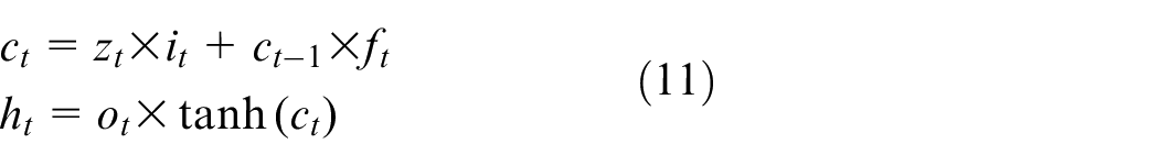
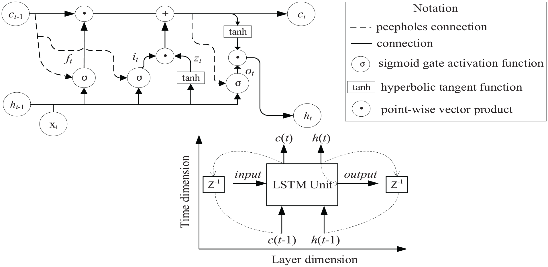
Schematic architecture of an LSTM unit. Top: Internal structure of LSTM. Bottom: External structure of LSTM (Z−1: one time lag).
The bottom plot in Figure 4 provides the reader with the external structure of an LSTM unit, from the point of system identification, it is preferable to treat it as a black-box module with a recurrent structure. Specifically, two dimensions are introduced to describe signal flow relations therein. In the time dimension, both cell state
Bidirectional LSTM network
It is interesting to note that a common feature of all above networks is that only previous context is utilized to calculate the current output, which to some extent poses limitations on the learning capability of the network. In order to overcome this limitation, the bidirectional RNN (BRNN) is proposed in Schuster and Paliwal
30
such that not only past sequence elements but future ones are taken into consideration. Unlike the standard RNN of the form (5), in BRNN the single hidden layer is replaced by a forward and backward hidden layer, and the backward hidden sequence
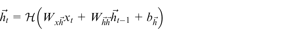
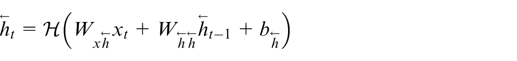
The bidirectional LSTM (BLSTM) is obtained by integrating BRNN and LSTM, 31 which has the property of memorizing long-span relations within a sequence in both directions. Since the forward part in BLSTM is identical to the LSTM unit introduced earlier, only the mathematical expression for backward one is given below, with reference to (8)–(10), it is derived as
where parameters in (11) are defined in the same fashion as those in (8) and (9), and the only difference lies in notations. Next, deep versions of two above LSTMs are given and used for the system identification purposes.
Deep design of LSTM for dynamic system identification
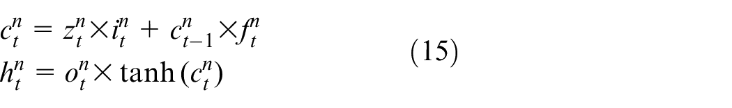
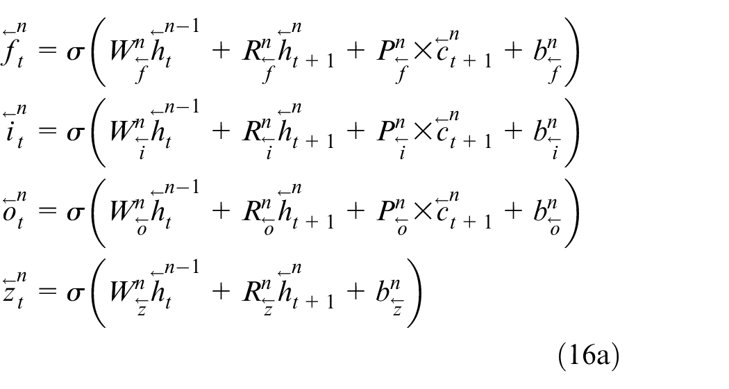
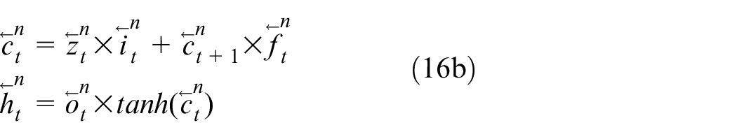
In this part, the design work of deep layered vanilla LSTM and BLSTM is given first, then the validity of using LSTMs for system identification is analyzed theoretically. As with the way of constructing deep RNN/NARX network, deep LSTMs are realized by cascading multiple LSTM (BLSTM) units. From the system identification viewpoint, each unit can be considered as a forced dynamic system of the form (8) and (9), and a DL-based LSTMs essentially corresponds to multiple forced dynamical systems that are connected in cascade, thus it is expected to have a powerful dynamics approximation capability. The nth layer of a deep LSTM network at time t is formulated as
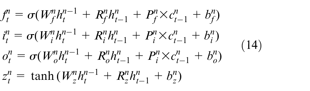
where the subscript signifies the time instance, for
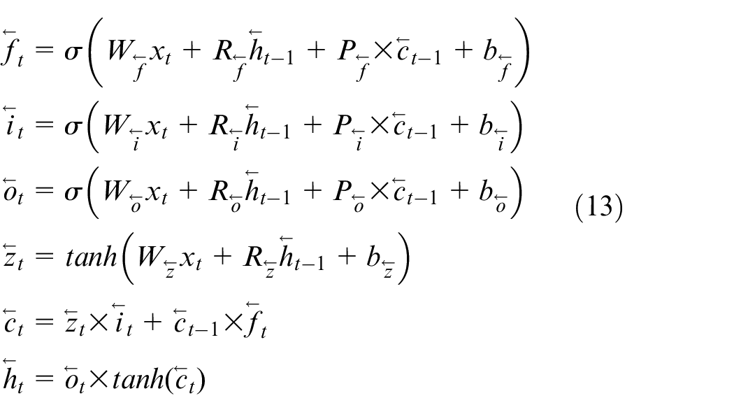
Likewise, a DL-based BLSTM is constructed by stacking BLSTM units introduced earlier, wherein the forward hidden layer sequence (
Two types of states are mathematically expressed as
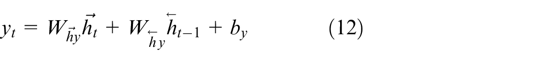
and the network response is calculated as
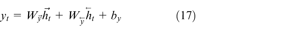
where
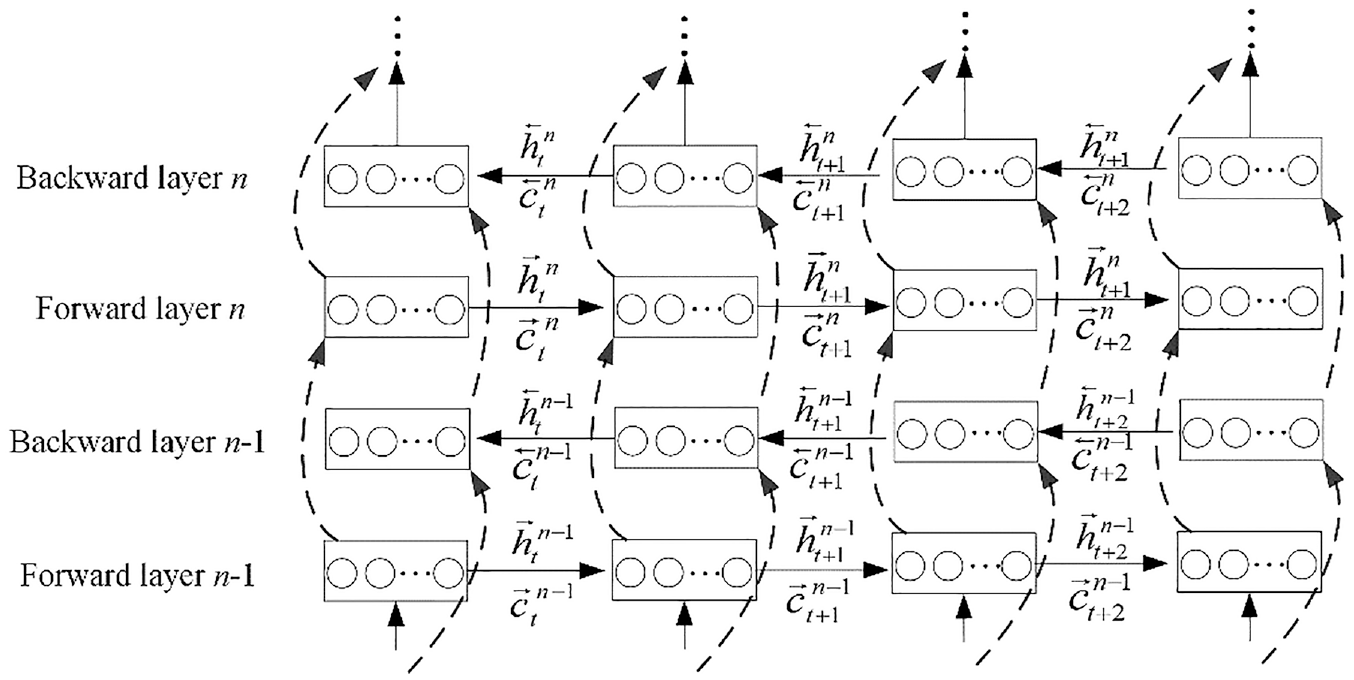
An unfolded deep learning-based BLSTM. The circular block in an LSTM unit denotes a memory cell.
Next, the identification capability of an LSTMs-based network is analyzed theoretically. It follows from (12) and (13) that there exist two types of states in an LSTM unit, namely a cell state
At this point, the focus is on identification system design of the FGD process. As mentioned earlier, the FGD process to be identified is an SISO dynamical system, with feeding flow of slurry
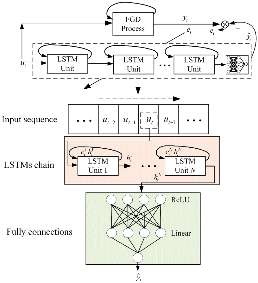
Identification system for FGD process consisting of a deep learning–based LSTMs network schematic.
Experimental results
In this section, all identification models described earlier are evaluated in an FGD context. For comparison purposes, representative models from other literature in this direction are also considered, and a quantitative assessment of each candidate model is performed.
Experimental condition
The simulation study carried out in this section is based on a real FGD process at a 600 MW coal-fired power plant, which is located in the province of Hebei, China. Operation data (i.e. flow of feeding limestone slurry and slurry pH value in the reaction tank) are obtained from the on-line data logging system, which records measurements within a fixed time interval per day. With a sampling time of 1 min, observations from January 3, 2022 to January 15, 2022 are obtained. With the outlier/missing data removal procedure is performed, the resulting dataset is divided into three parts: 80% for training and 20% for testing. Here a distinction is made between two types of data sets, a training set is utilized for the model development purpose, while the test set plays the role of giving the final evaluation on the generalization performance of a certain model.
Network architecture and experimental design
In our experiment, all identifiers described earlier are evaluated including: (i) NARX-based network in equations (3) and (4), (ii) recurrent network (RNN) in equations (6) and (7), (iii) LSTM network in equations (12) and (13), and (iv) BLSTM network in equations (14) and (15). Furthermore, identifiers come from past works in FGD process modeling direction are also involved, they are ARX model in Li et al.,
32
cascade forward neural network (CFNN) in Di Capaci and Scali,
33
NARX model in Li et al.
34
and RNN in Wu et al.
35
In all cases, parameters are estimated by minimizing the loss
The hyper-parameters play an essential role in the performance of a model, and the best-performing model depends upon the optimal combination of hyper-parameters. Each experimental model discussed in this section comprises multiple hyper-parameters (e.g. key hyper-parameters in a vanilla LSTM include: memory cell number, dropout rate and the number of stacked LSTM blocks). As a consequence, it is essential to choose an appropriate method to optimize hyper-parameters. Here the random search combined with five-fold cross-validation technique is adopted to optimize hyper-parameters in each experimental model. Due to the fact that multiple hyper-parameters are covered for each experimental model, the grid search and manual search method become computationally infeasible. Additionally, the random search possesses practical merits of grid search and shows more efficiency for hyper-parameter optimization in a high-dimensional search space. 37 As a consequence, the random search that makes use of a randomized search of the hyper-parameter space to minimize training time while ensuring performance is adopted. Besides, according to Browne, 38 the cross-validation technique has the benefits of making efficient use of data and preventing the over-fitting problem. In five-fold cross-validation, a training set is partitioned into four subsets for training and one subset for evaluating the performance of established model. This process is repeated for five times to obtain five different combinations and each subset is chosen once for validation. Then the results are averaged to obtain the final cross-validation result. To facilitate the performance evaluation of each experimental model, two evaluation metrics mean squared error (MSE) and mean absolute percentage error (MAPE) are introduced, they are written as
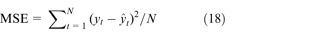
where
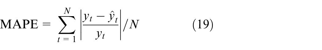
(1) Estimate the range of each hyperparameter in an experimental model with several preliminary runs, and assign corresponding values within it to build the hyper-parameter space.
(2) Search the hyper-parameter space using the random search technique, and the search is performed for a maximum of 50 iterations.
(3) Train the experimental model with searched hyper-parameters using five-fold cross validation, and evaluate its cross-validation performance using the metric MAPE defined in equation (17).
(4) Compare all obtained results and hyper-parameters of the best one (i.e. the lowest cross-validation MAPE score) are selected, which are then used to train the model on the whole training set.
(5) Test the established model on the test set.
Figure 7 depicts the whole procedure for hyper-parameter optimization for our experimental models. The hyper-parameter information of experimental models, namely the selection range and specific values of hyper-parameters, are presented in Table 1. Following the above procedure for hyper-parameters optimization, optimized hyper-parameters of each experimental model can thus be determined, which are also listed in Table 1.
Diagram that illustrates the hyper-parameters optimization process.
Hyper-parameters selection ranges and optimized values for deep learning experimental models.
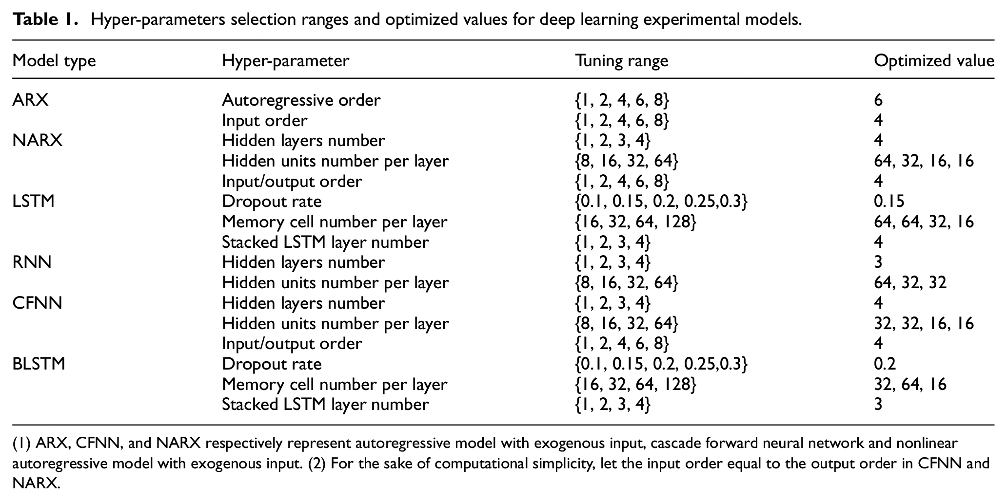
(1) ARX, CFNN, and NARX respectively represent autoregressive model with exogenous input, cascade forward neural network and nonlinear autoregressive model with exogenous input. (2) For the sake of computational simplicity, let the input order equal to the output order in CFNN and NARX.
Modeling results and discussion
In this part, with the experimental design stated above, all candidate models are tested sequentially. For notational brevity, suppose there exists m0 input variables and m
L
outputs, a family of neural models with m
l
units at the lth layer is denoted as
Case 1: ARX model.
Case 2: NARX model
Case 3: RNN model
Case 4: CFNN model
Case 5: LSTM and BLSTM model.
Case 1: ARX model
As the most commonly used linear dynamic model, ARX was adopted to identify the FGD process. Besides it can provide a benchmark for comparing model performance in other cases. According to the order range listed above, a total of 4 ARX models are constructed. It is found that when the autoregressive order and input order are respectively determined as 6 and 4, the model has the lowest cross-validation MAPE score and hence is selected. Performance of the selected model on test set is shown in Figure 8(a) below, and the resulting MSE and MAPE respectively reach high values up to 0.177 and 0.1827, implying ARX model is not a desirable choice.
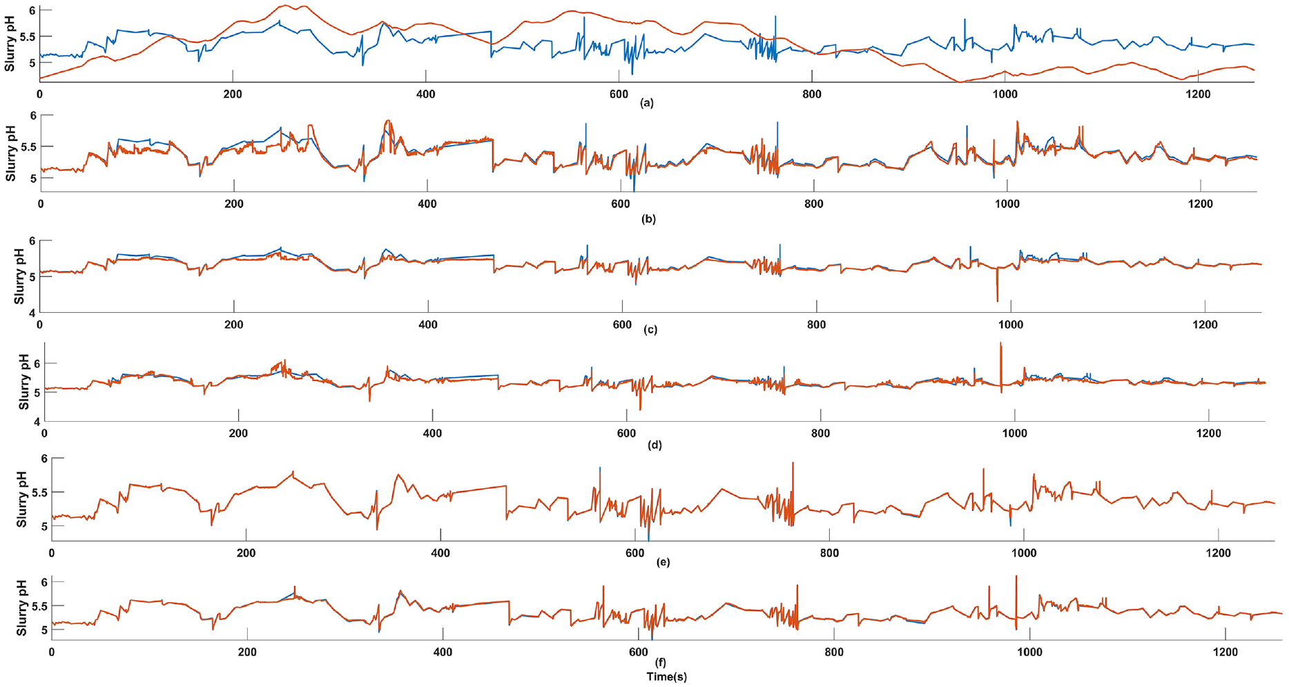
Identified results of different models. Red line: model output. Blue line: target: (a) ARX, (b) NARX, (c) RNN, (d) FCNN, (e) LSTM, (f) BLSTM.
Case 2: NARX model
In this case, NARX model is utilized to perform the identification task, and networks with all possible hyper-parameter combinations are separately trained and evaluated on validation set. Following the procedure stated in experimental design part, the model belongs to
Case 3: RNN model
To evaluate RNN model’s identification capability for FGD process, the same procedure is followed to search for the optimal network architecture. The searching result indicates that a high proportion of MSE values range between 6 × 10⁻³ and 7 × 10⁻³, and the optimal architecture corresponds to the minimum among all results (3.2473 × 10⁻³) and is determined as
Case 4: CFNN model
In this case, CFNN model in Alkhasawneh and Tay
40
is considered. As before, networks with different parameter combinations are trained and evaluated on validation set. By comparing all results, the model belongs to
Case 5: LSTM-based models
In this case, the FGD process is identified by LSTM model and its variant BLSTM model. Comparing with identifiers utilized above, LSTM and its variant have strong capability in capturing long range temporal dependencies between input and output sequences. With parameter combinations defined above, a total of 120 candidates are trained and evaluated on validation set, eventually the one with 64, 64, 32, and 16 memory cells in each stacked unit is chosen; While for the BLSTM model, the number of stacked units is 3, with 32, 64, 16 cells in each unit. As is clearly seen from Figure 8(e) and (f), the real slurry pH and model output are almost indistinguishable, suggesting the remarkable identification performance of two LSTM-based identifiers.
Aiming at comparing the performance of shallow network (single-layered architecture) and deep-layered one (refer to the case where hidden layer number is equal to or greater than three), in Table 2 we list best selected models in Case 1–5, along with their MSE/MAPE scores on training and test set, besides average results on validation set are also included. According to results shown in Table 2, two conclusions can be drawn: (1) Deep learning-based architecture enables improvement of model’s identification performance. Specifically, all deep learning models have lower MSE and MAPE scores on the test set as compared to their shallow structure counterparts, and the largest reduction rate for MSE and MAPE reach 81.90% (NARX) and 84.15% (LSTM), respectively. (2) The deep-layered BLSTM model performs best among all experimental models, and it achieves the lowest MSE value of 4.352 × 10⁻⁴ and lowest MAPE value of 0.0010, implying it has the minimum absolute and relative error defined in terms of actual and predicted values, and consequently deep-layered BLSTM is the most suitable model for identifying the studied flue gas desulfurization process.
Comparison results for different shallow/deep models.
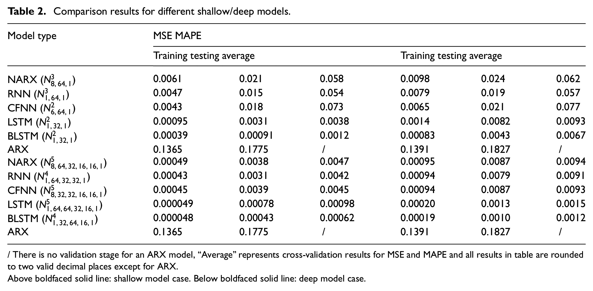
/ There is no validation stage for an ARX model, “Average” represents cross-validation results for MSE and MAPE and all results in table are rounded to two valid decimal places except for ARX.
Above boldfaced solid line: shallow model case. Below boldfaced solid line: deep model case.
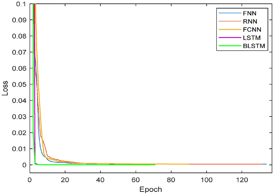
The training objective function (also referred as training loss) to be minimized is chosen as the mean squared error, and the training loss related to the epoch number for each experimental model is shown in Figure 9, which is a convenient tool for observing the learning degree of a model during the training process. 41 It is found that all losses decrease rapidly at the early stage of training, then vary little and converge to a small value after some epochs, and main distinctness among different models lies in the convergence epoch and convergence value.
Comparison of learning curves of different neural models.
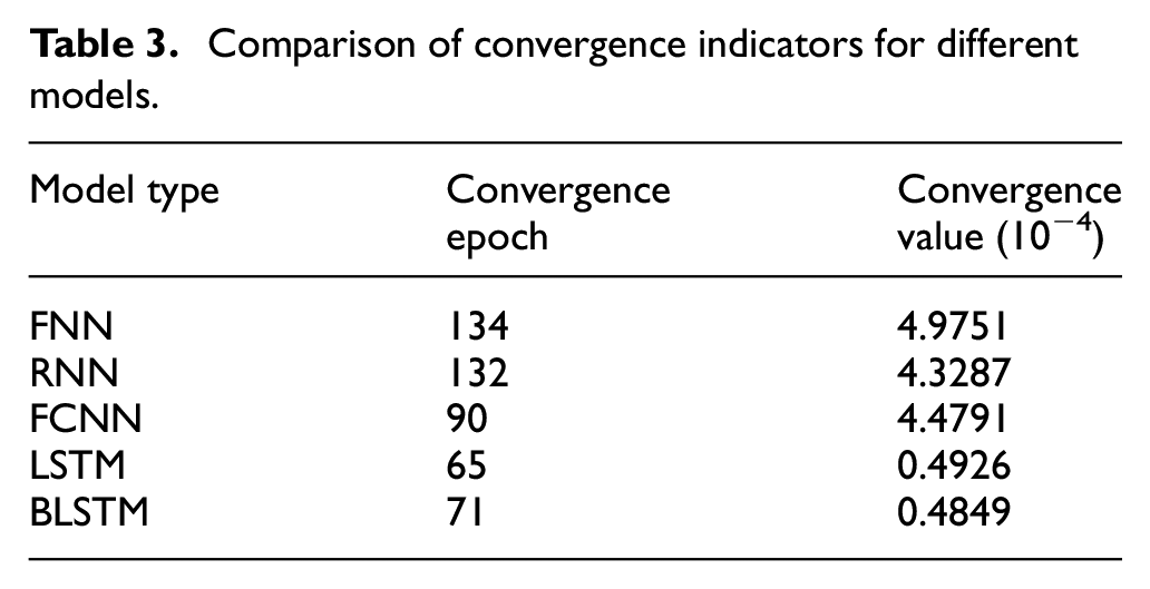
Table 3 shows details concerning above two convergence indicators for different models, we can clearly observe that LSTM and BLSTM respectively have the minimum convergence epoch and convergence value. More specifically, it takes 65 epochs for LSTM to converge to 4.926 × 10⁻⁵, meanwhile 71 epochs is required for BLSTM to reach the loss of 4.849 × 10⁻⁵.
Comparison of convergence indicators for different models.
Conclusion
In this work we attempt to explore the feasibility of applying DL-based technique to the system identification problem. FGD process, as a representative non-linear dynamic system with high level of complexity, is taken as the case study. We first analyzed the relationship between DL and system identification, and presented deep form of commonly used neural identifiers and particularly LSTMs. It is found that LSTMs have structurally advantages when used for system identification. Then systematic experiments are performed to evaluate the identification performance of selected identifiers in an FGD context. According to experimental results, it is found that MSE and MAPE for the best-performing deep BLSTM model respectively achieve 4.352 × 10⁻⁴ and 0.0010, and in comparison to those obtained in the second best deep LSTM model, the MSE and MAPE scores are decreased by 44.87% and 23.08%, respectively. Additionally, it is concluded that modeling performance is improved significantly when deep-layered structure is introduced, and LSTM/BLSTM is particularly suited to identify the FGD process, since they benefit from rapid learning speed and high identification accuracy. The integration of advanced DL network and system identification shows great success in our paper. In future investigations, a further step will be made by incorporating the controller design part.
Footnotes
Declaration of conflicting interests
The author(s) declared no potential conflicts of interest with respect to the research, authorship, and/or publication of this article.
Funding
The author(s) disclosed receipt of the following financial support for the research, authorship, and/or publication of this article: This study is supported by the National Natural Science Foundation of China (62373012 and 62303025).
Data availability statement
Data sharing not applicable to this article as no datasets were generated or analyzed during the current study.