
Abstract
A cutting tool’s remaining useful life is what is left for a tool, at a particular working age, in order to reach a pre-specified level of acceptable performance. The prediction of remaining useful life is crucial in order to decrease the scrapped products or the unnecessary interruption of the machining process in order to replace the tool. Consequently, the accuracy of its estimation affects the cost of machining, particularly when the product’s material is very expensive. In this article, the remaining useful lifes of 25 identical tools are estimated during turning titanium metal matrix composites. These composites are extensively used in aerospace and aviation industries. Accurate estimation of the remaining useful life has positive impact on product quality in terms of producing the required specifications. In this article, experimental data are gathered, and the proportional hazard model are used in order to model the tool’s reliability and hazard functions with EXAKT software and then the remaining useful life curves are developed for different machining conditions, namely, the cutting speed and the feed rate. The use of the proportional hazard model is validated using a normalization process and Kolmogorov–Smirnov test. The proportionality assumption is verified using log minus log plot. The final result is the development of the curves that represent the tools’ reliability and the remaining useful life for different machining conditions of the titanium metal matrix composites.
Introduction
The characteristics of titanium metal matrix composites (Ti-MMCs), such as low weight, high mechanical and physical properties, and high stiffness and strength, have brought them up as useful materials in different industries. 1 Although very expensive, Ti-MMCs are a new generation of materials which have proven to be viable in various fields such as biomedical and aerospace industrial. For these reasons, finding the cutting tool’s remaining useful life (RUL) while machiningTi-MMCs is important in order to decrease the scrapped products or the premature replacement of the tool and consequently the cost of machining. The estimation of the cutting tool’s RUL during the machining of Ti-MMCs is more difficult than other metals because of the high wear resistance which causes high wear rate on the cutting tools and also because the nonhomogeneous composition and abrasive properties of the reinforcing particles; the cutting tool confronts particles and matrix whose responses to machining process could be completely different. The machinability ofTi-MMCs is often considered poor because of the material’s characteristics, such as low thermal conductivity and high strength at high temperatures. 2
The RUL is generally defined as the expected useful life left for a tool at a particular time of operation. 3 Knowing the RUL has an economic impact, since replacing the tool earlier than necessary will cause the loss of valuable resources and time, while replacing the tool later will result in defective products. 4 The cutting tool’s RUL estimate captures the output of a stochastic process, which is the wear increase, by providing a probabilistic estimate of the tool life as the cutting conditions change. Consequently, a replacement decision can be made in order to avoid unplanned tool failure.
Many researchers tried to estimate the RUL of some cutting tools. For example, Si et al. 3 presented an exclusive review of the statistical data–driven approaches which are used to estimate the RUL. Sikorska et al. 5 discussed the issues that need to be considered when selecting the suitable approach for estimating RUL. The authors also presented a classification of appropriate prognostic models for predicting the RUL of engineering assets. Banjevic 6 discussed the importance of calculating the RUL in industrial applications. Aramesh et al. 7 estimated the RUL of cutting tools during turning Ti-MMCs using the reliability function which is based on a Weibull distribution. In their article, the authors assumed three stages of tool wear in order to find the model that best represents the obtained experimental results. Baruah and Chinnam 8 used hidden Markov models (HMMs) for carrying out diagnostic and prognostic activities for metal cutting tools during drilling process. HMMs were also used with the sensor signals emanating from the machine in order to identify the degradation state of the cutting tool and estimate the RUL. Wang and Wang 9 used continuous hidden Markov model (CHMM) in order to calculate the RUL during a milling process. The authors considered the cutting forces as the monitoring signals that indicate the tool wear state. The authors also used a Gaussian regression model in order to predict the milling tool’s RUL. Gokulachandran and Mohandas 10 presented two approaches for the prediction of remaining life of carbide-tipped tools: a regression model and an artificial neural network and then the results of both models were compared.
The main differences between this article and the previous researches, which are presented in Banjevic 6 and Aramesh et al., 7 are as follows:
The developed model considers variable machining conditions, while in Banjevic, 6 the study is conducted under constant machining conditions;
The developed model is based on the proportional hazard model (PHM) which reflects the effect of the machining conditions on the RUL, while in Banjevic 6 and Aramesh et al., 7 the two articles considered the Weibull distribution only and did not take into consideration the machining conditions;
The obtained results of this article are the curves of the RULs which are estimated as functions of the machining conditions, while in Banjevic, 6 the outputs are the sojourn time and the transition times between the wear states;
The developed curves are based on modelling a nonhomogeneous Markov model, which represents a stochastic process with transition matrix, while in Baruah and Chinnam 8 and Wang and Wang, 9 HMMs are considered.
The objective of this article is thus to develop the RUL curves of cutting tools during turning Ti-MMCs under variable conditions. In this study, Ti-6Al-4V is selected among the different Ti-MMCs alloys. The PHM is used to calculate the tool’s reliability and hazard functions and estimate the RUL. The cutting speed
In section ‘Description of the experiment’, the description of the experimental setting is presented. In section ‘Model development’, the PHM for a tool operating under variable conditions is introduced. In section ‘Model validation’, the validation procedures for the obtained PHM are presented. In section ‘RUL’, the theoretical and mathematical basis for the estimation of the RUL is given. Concluding remarks are given in section ‘Conclusion’.
Description of the experiment
Equipment
At the computer numerical control (CNC) turning centre of Polytechnique Montréal, a six-axis Boehringer NG 200 is used in order to conduct the experiments. The used CNC turning centre has live tooling, programmable steady rest, Y-axis, and C-axis.
Tool material
Seco TH1000–coated carbide grade is used. TH1000 is a TiSiN-TiAlN nanolaminate physical vapour deposition (PVD)-coated grade which is produced by Seco global company. Its coating structure includes a nanolaminate PVD top layer for maximum toughness and high chipping resistance. TH1000 is highly resilient to edge fracture which is the kind of wear that typically occurs when turning hard surfaced materials such as MMCs. The experimental setup is shown in Figure 1.
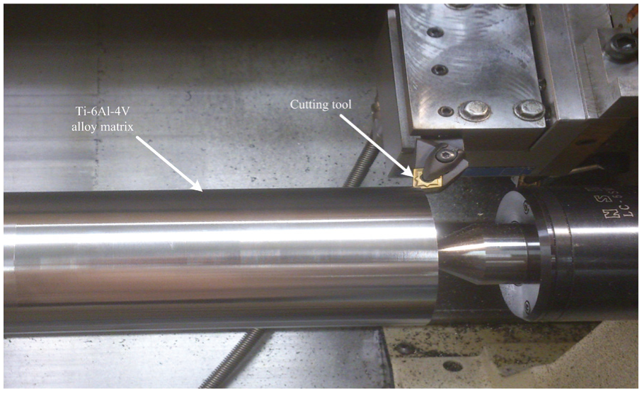
Experimental setup.
Workpiece material
A cylindrical bar of Ti-6Al-4V alloy matrix reinforced with 10%–12% volume fraction of TiC ceramic particles is used for turning. Ti-MMC alloys have superior mechanical and physical properties when compared to the conventional materials. Ti-6Al-4V is selected among the Ti-MMC alloys because of its high strength and stiffness, high fracture toughness, and good deformability at high temperature. 11 The density of conventional Ti-MMCs is 4040 kg/m3, and the stiffness is 200 GPa. 12
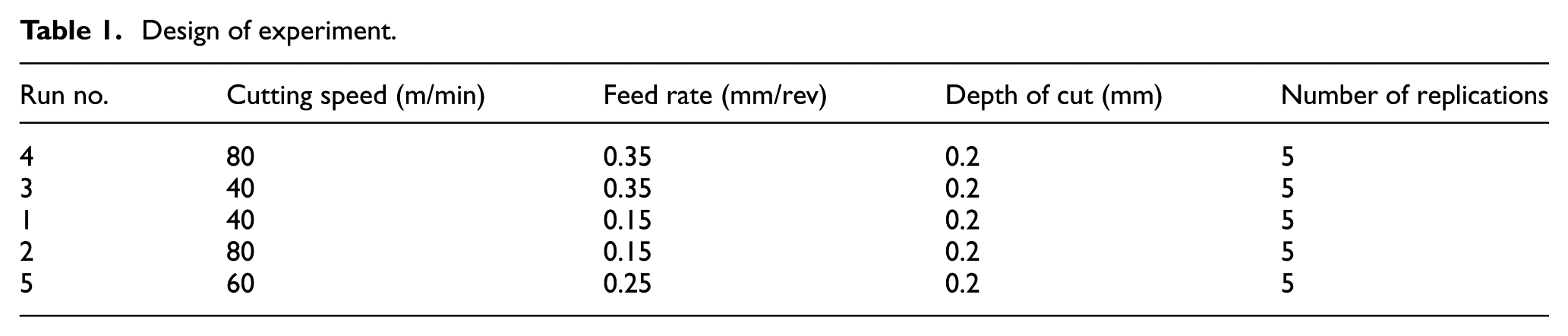
Design of experiment
Design of experiment (DoE) techniques were implemented to investigate the influence of factors on the predicted output result.
13
The control conditions such as cutting speed and feed rate were used in DoE in titanium metal cutting research.
14
The full factorial designs with two factors, two levels (
Design of experiment.
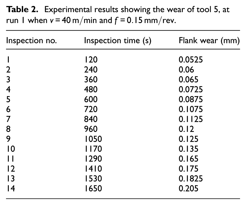
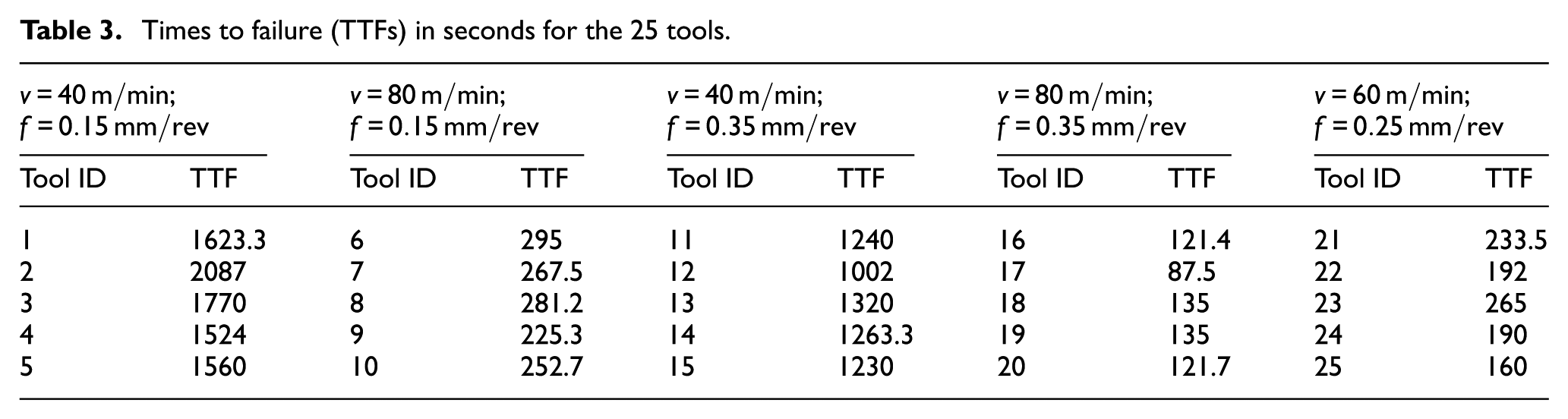
Each replication uses a new tool on which sequential inspections are performed in order to measure the wear. An Olympus SZ-X12 microscope is used to measure the flank tool wear at discrete points of time through inspections. This procedure continues until the cutting tool fails and becomes dull and no longer operates within acceptable quality. The predefined threshold (VBBmax = 0.2 mm) is set to define the tool failure. For example; the experimental data of run 1 and tool 5 is shown in Table 2. The time to failure (
Experimental results showing the wear of tool 5, at run 1 when
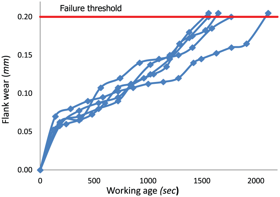
Tool wear measurements for five tools at run 1 with
Times to failure (TTFs) in seconds for the 25 tools.
Model development
The tool life of a cutting tool is a random variable, and its degradation is a stochastic process that depends not only on the age of the tool but also on the covariates which describe the machining conditions.
15
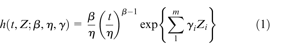
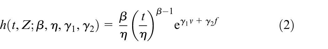
In the PHM, the failure rate is modelled as the product of a baseline failure rate, which is dependent only on the age of the tool and an exponential expression which is the linear sum of
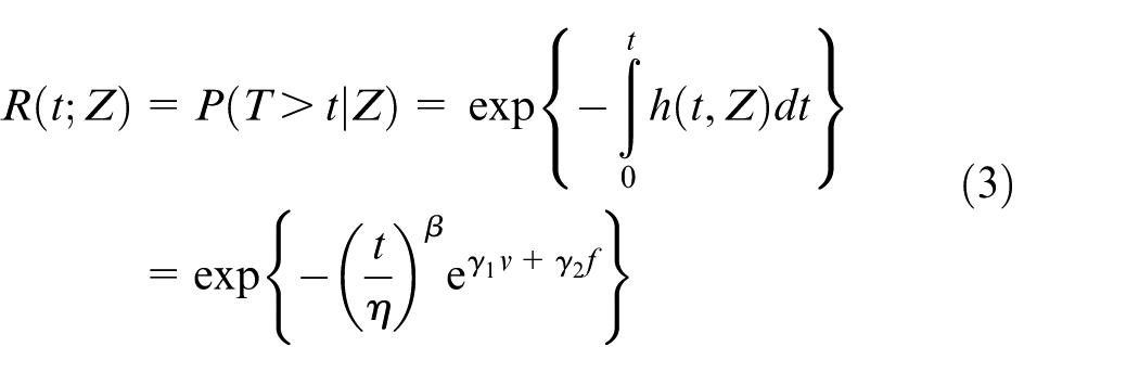
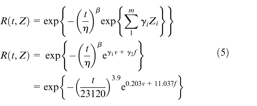
The hazard function formulation with the PHM leads to a corresponding survival function formulation as shown in equation (3). This survival function formulation
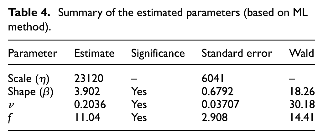
In order to estimate the parameters
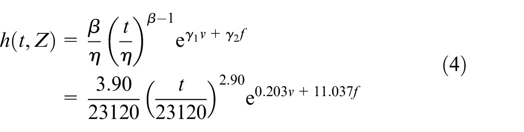
It is to be noted that the covariate parameter values γ1 = 0.203 and γ2 = 11.037 do not represent the effects of the conditions on the hazard rate, because these values are not normalized and depend on the measurements’ scales. A small value for
Summary of the estimated parameters (based on ML method).
Based on equation (3), the reliability curve is plotted for each of the combinations of feed at 0.15, 0.25, and 0.35 mm/rev and speed at 40, 60, and 80 m/min as shown in Figure 3. By comparing between these curves, the effect of the machining conditions on the probability of failure is shown. For example, the higher effect of the cutting speed, in comparison to the effect of the feed rate, is clear when comparing between the reliability curve 1 and the reliability curve 7, where both curves have the same feed rates,
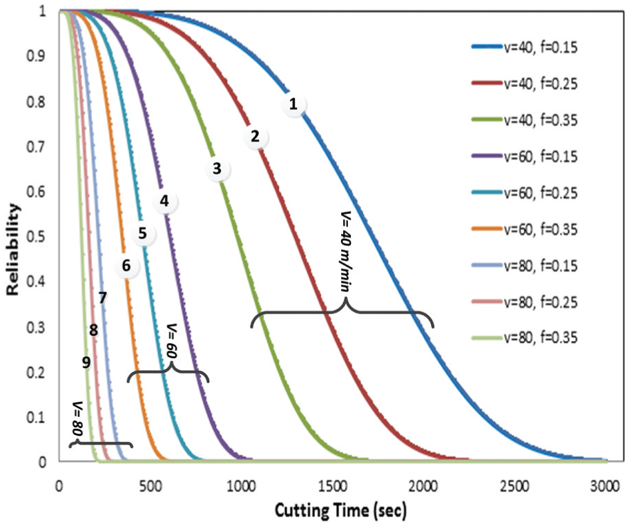
Reliability functions for nine combinations of speed and feed in the given range.
Model validation
The objective of this section is to present three methods that are used in this article in order to validate the use of the PHM in modelling the degradation of the cutting tool condition due to wear. The results of this validation prove that indeed the PHM represents adequately the degradation of the tool due to wear. In the following subsection, the three methods are presented.
Normalization
Intuitively, the cutting speed’s effect on the cutting tool life should be greater than the feed rate’s effect. To prove this intuitive assertion, the cutting speed and the feed rate effects are calculated using a simple normalization procedure. The normalization is used to adjust the values measured on different scales to a notionally common scale. Since the cutting speed and the feed are in the range
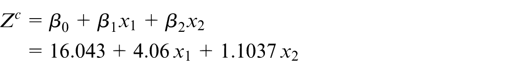
where
K-S test
K-S test is originally used as a test of equality of continuous, one-dimensional probability distributions that can be used to compare a sample with a reference probability distribution. This test can also be used to test the goodness of fit. K-S test is used to validate the model by evaluating its fit. The test checks the null hypothesis that the cumulative hazard function, which is
Summary of goodness-of-fit test results.
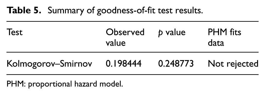
PHM: proportional hazard model.
Main PHM assumption
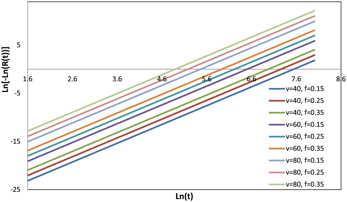
The main assumption underlying the use of the PHM is that the change in the tool wear rate, which is the change in the rate of degradation, is proportional to the change in the covariate values. This can be shown graphically in Figure 4.
Logarithmic reliability function plot.
Figure 4 gives the logarithmic reliability function plot which shows clearly that indeed the assumption of proportionality is satisfied since the combination values of speed and feed produce parallel lines in the log minus log plot. These lines should be parallel, and the distance between the curves should remain proportional across the time. 22 Figure 4 shows the analysis of the logarithmic reliability function (log minus log plot) based on equation (3). The linear equation for each speed–feed combination is as follows
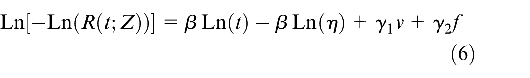
The logarithmic reliability function in equation (6) is linear in
RUL
The RUL at time
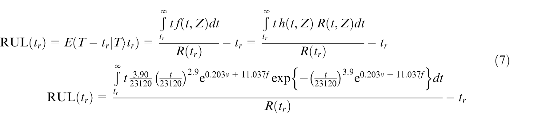
At time
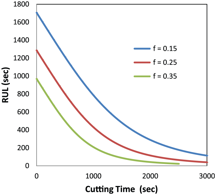
RUL estimation when
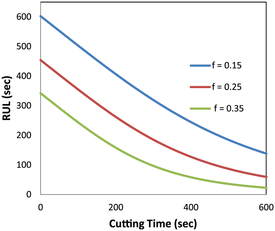
RUL estimation when
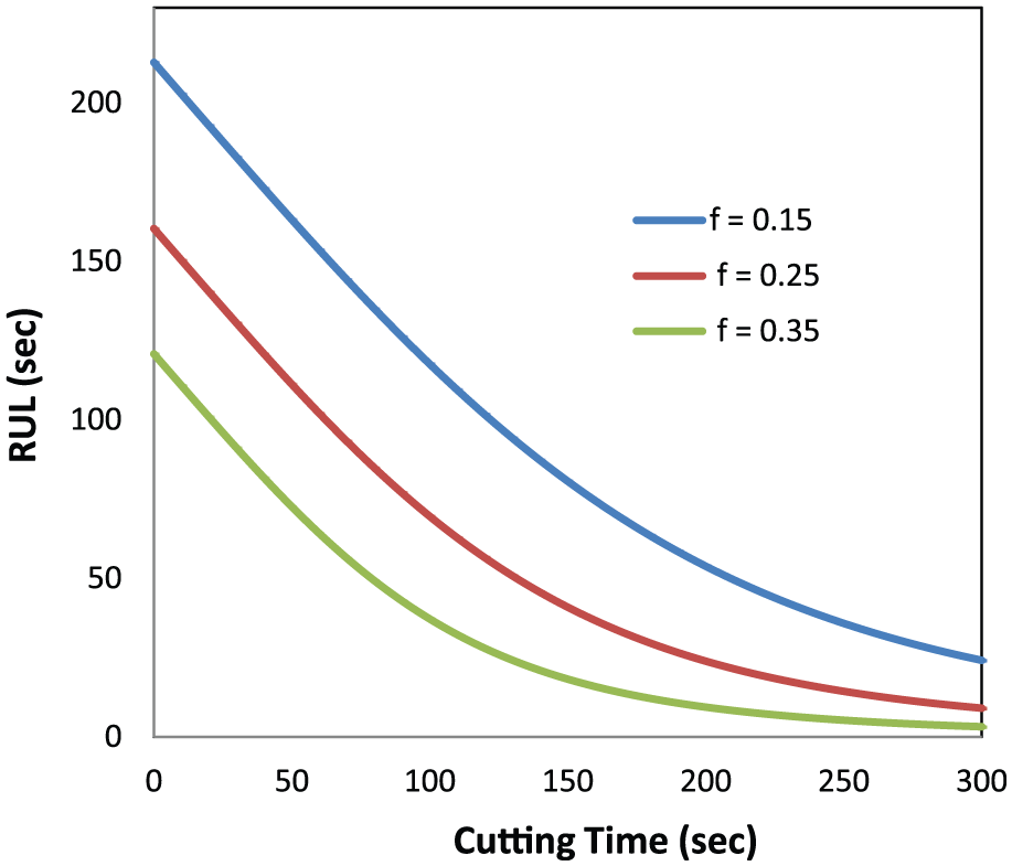
RUL estimation when
It is to be noted that the RUL, which is also called the mean residual life, is an estimation of the mean remaining life. As such, its value is based on the conditional probability that the tool will live until time
Similar to the RUL charts that are given in Figures 6 and 7, RUL charts were obtained in some articles for other applications. For example, In Elsayed, 26 the author presented the charts of the reliability function and the RUL using an estimated Weibull distribution for a furnace tube failure, with the scale parameter depending on the operating temperature. The temperature is a time-independent covariate, which is set at a specific value at the beginning of the tube’s life. Also, In Wang et al., 27 the authors presented the graphs for reliability function and the RUL using PHM and Monte Carlo simulation method. Four degradation states of equipment were considered when the RUL graphs were drawn. In Banjevic and Jardine, 28 the authors presented the graphs for reliability function and the RUL using Weibull PHM. The RUL charts were obtained for transmission systems of large transporters from a mining company. The wear metal iron is the significant covariate, and the transmission’s oil analysis history is time dependent.
One of the most useful aspects of the RUL charts is the ease of using them in the machining workshops. These charts can be built for any kind of material and tool. The procedure starts by designing, performing some experiments, and the observation of the events of tools’ failures by sequential inspections. The data concerning the covariate values is collected in order to build the PHM by estimating the parameters. The model is validated by checking the proportionality of the hazards and the K-S goodness-of-fit test. Finally, the RUL charts are obtained under different machining conditions.
The difference in the experimental results and results obtained from the developed model is presented in Figure 8 when
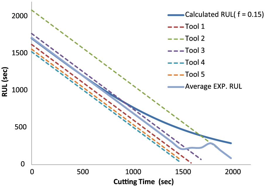
Experimental and calculated RUL at
Conclusion
During turning Ti-MMCs under variable machining conditions, the experimentally collected data were used to construct the PHM which takes into consideration the TTFs and the effects of the external conditions. The introduction of the PHM as a viable model to represent the degradation phenomena of a cutting tool and the validation of this model with three different techniques are presented. The estimation of the RUL of a cutting tool as a function of the machining conditions is developed. The charts for the RUL of Ti-MMCs under different machining conditions are constructed. The future work aims at incorporating the sensors’ data about the uncontrollable variables, which are the forces and the torque, in the PHM. It is also planned to create the RUL curves in an online system in order to estimate the cutting tool RUL autonomously. The RUL curves will be generated and updated at each inspection time
Footnotes
Appendix 1
Declaration of conflicting interests
The author(s) declared no potential conflicts of interest with respect to the research, authorship, and/or publication of this article.
Funding
The author(s) received no financial support for the research, authorship, and/or publication of this article.