
Abstract
In this article, a novel optimization method for beam–plate structure is proposed based on two optimization levels, including the topology optimization and the section optimization. First, the optimal topology of structure with fixed material and dimensions of design domain is obtained using bidirectional evolutionary structure optimization method, and then, the section optimization is made to produce final optimal solution based on response surface model. In order to deal with beam–plate structures, the traditional bidirectional evolutionary structure optimization method is improved using cubic box as the unit cell instead of solid unit to construct periodic lattice structure. To handle irregular structural element layout produced in bidirectional evolutionary structure optimization method, section conversion process is employed to smooth the edges of sections; in this way, the manufacturability of optimal solution will be significantly improved. To determine the section parameters, response surface method is used to perform the section optimization, and the structure mass is further reduced. One example of cantilever beam structure design is provided and discussed. The applied two-stage optimization procedure resulted in 86 iteration steps to obtain the optimal topology, and a further decrease in 2.65% mass on the basis of optimal topology, which shows that the proposed method has advantages on convergence rate and computational cost.
Keywords
Introduction
This research is motivated by the need for minimizing the weight of a series of beam–plate structures. Beam–plate structures are widely used in many engineering fields such as civil engineering, bridge engineering, ship and offshore structures, and heavy machinery. Typical beam–plate structure system includes beams, girders, and plates. It is known that for various functional requirements such as providing enough working area, bearing static or dynamic loads, and retaining good sealing ability, flat panel is the first adopted structural component. Because a thin panel is relatively weak under complicated load cases, and it is very uneconomic to improve the stress performance only by increasing thickness of panel; however, excessive deformation can be avoided and much lighter weight can also be achieved by adding longitudinal and transverse members, namely, beams and girders. With good manufacturability and stress performance, this topological form has been used for centuries except in very special case. Figure 1 shows some typical beam–plate structures.
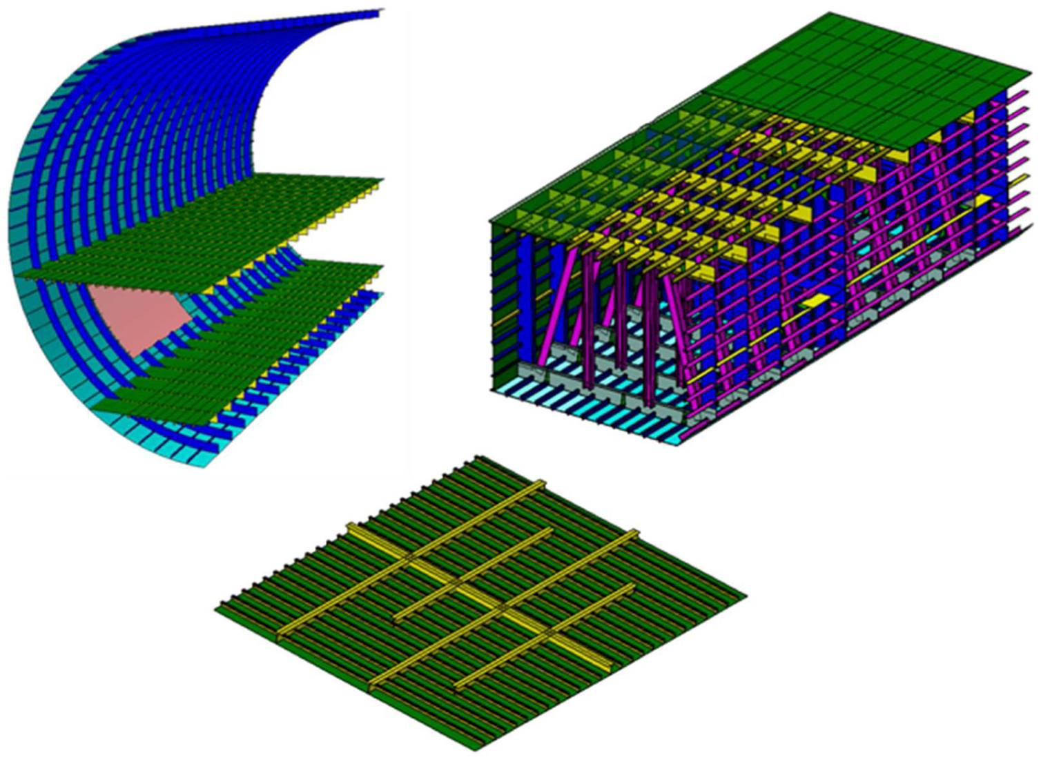
Typical beam–plate structures.
Due to the relatively fixed topological form, beam–plate structure can be described by several categories of parameters covering size, section, and topology level. For example, the length, width, and height describe the size of structure; plate thicknesses and beam sections are parameters of section level, while the number and spacing of beams and girders describe the topology. Beam–plate structure can be considered that be composed of stiffened plates; the thickness of each plate may vary. Moreover, when the size of beam–plate structure grows, there may be several different plate thicknesses on one plane.
With the development of optimization methods, previous researches1–6 on beam–plate structure optimal design had made great achievements; however, many simplifying works had to be pre-processed to decrease the calculation scale and cost such as using one section to represent multiple structural members. Nonetheless, there are few changes in topological form among the existing works. These factors limit access to global optimization solution. It is also difficult to balance the conflict between increasing calculation efficiency and determining a proper design space. As shown in Figure 2, using of line or curve to express the locations of beams or girders, extruding the lines or curves in the direction perpendicular to the plate plane can form a feasible solution of beam–plate structure design, while the combinations of lines or curves can be limitless, which indicates that there can be infinite feasible solutions if the classical topological form is abandoned.

Comparison between innovative and conventional topological forms.
In recent decades, many heuristic methods such as evolutionary structure optimization (ESO) method,7,8 bidirectional evolutionary structure optimization (BESO) method,9,10 and metamorphic development (MD) method 11 have emerged and have made great progress on continuum structure optimization; among these, BESO is the most representative one. Many examples using BESO demonstrated the ability to find the best topological form, and the optimum usually presents a novel but highly efficient topology in contrast to the traditional topology. It is a simple idea to apply BESO in optimization of beam–plate structure, but it is found that satisfied results hardly can be achieved if the conventional solid cubic design domain is used. Through investigating the initial design domain and mesh type of BESO for optimization problem of beam–plate structure, lattice architecture is adopted to form initial design domain. A few numerical examples are considered using different levels of finite element (FE) grids, and conclusions regarding convergence and the element size effect are reached.
Based on the modified BESO method, an innovative optimization method for beam–plate structure is proposed. Compared to most existing methods for beam–plate structure optimization, the proposed method in this article has three unique features. First, the optimal topological form generated by BESO may be much different from the conventional topological form. Second, optimization problem of topology level and section level is considered, which broadens the application range of the proposed method. Third, in the proposed method, the type of the basic unit structure is considered as a design variable. It may further enhance the mechanical performance of designed products. In section “Basic concepts,” some basic concepts in the proposed method are introduced. Based on these basic concepts, the proposed method of beam–plate structure optimization is presented in section “Overall process of BESO-based beam–plate structure optimization method.” In section “Case study,” a case study is provided to validate this proposed method. Finally, this article is wrapped up with the conclusion and future prospects.
Basic concepts
Beam–plate structure optimization without topology restriction
The main purpose of this article is to find that potential topological forms may have better structural property and better distribution of materials than conventional topological forms for beam–plate structure design. Without the restriction of topological form, the scale of beam–plate structure optimization problem will become much larger. Generally, the design variables of conventional topological form are discrete variables; therefore, some combinatorial optimization methods can be used. However, if the restriction of topological form is no longer considered, some design variables may be continuous, and even the number of design variables cannot be estimated precisely; then, combinatorial optimization method cannot be any more effective, which produces a need for more powerful optimization method.
BESO method is a FE-based topology optimization method; 12 its principle is that inefficient material should be iteratively removed from the initial design domain, while efficient material should be simultaneously added, whereas ESO can only remove elements, which may cause permanent, irreversible change to previous state, and then, the final solution could be non-optimal. As an extension of ESO method, BESO has two advantages over ESO. First, it is more robust for preventing prematurely removing elements. Second, compared to ESO, using an over-sized ground structure, BESO can be computationally more efficient, as it can start from a simple initial design and thus decrease the scale of FE model. Although a ground structure still can be specified alternatively, BESO has the flexibility to grow the structure without bounding the design domain. BESO has demonstrated its strength in solving stress-based problems with stiffness/displacement. A simple idea is to apply ESO/BESO methods to beam–plate structure optimization.
Full details of BESO procedures are presented by Yang et al. 9 The procedure for solving stiffness/displacement problems can be described as follows:
Define an initial design domain with boundary and loading conditions; the initial design domain is usually a simple structure connecting all supports and loads.
Perform FE analysis to obtain information on displacement and/or stress.
Perform sensitivity analysis. Pick out the most efficient elements and the least efficient elements. Add elements around the most efficient ones and remove the least efficient elements. The performance index (PI) should be calculated to measure the quality of the design.
Repeat steps 2 and 3 until the structure reaches the prescribed weight/displacement; if the PI starts to increase for some iterations, then remove more elements than are being added.
How to apply BESO method to beam–plate structure optimization
Started from two-dimensional (2D) age, ESO/BESO methods have entered into three-dimensional (3D) stage. It is a common practice of 3D BESO method to create the initial design domain using brick element and add or delete elements to achieve the optimal topology. The optimal designs of conventional 3D BESO method usually have an innovative shape consisting of various strangely structural members. Because the edges of brick element are orthogonal, the edges of optimal topology are jagged that need to be smoothed to make the fabrication process more feasible. As for the manufacturability of the optimal structure of 3D BESO method, the smaller is the size of the structure, the harder is the manufacturing process, which limits the application of 3D BESO method into practical use.
However, with the successful application of additive manufacturing technology, the optimal structure of 3D BESO method can be made much more easily than before, but it may be not suitable for replacing beam–plate structure under some circumstances. Take the steel structure of liquid container; for example, the effective thickness keeps decreasing due to various damage types, such as corrosion and cracking, and it is very important to process inspection, maintenance, and repairing during the whole life cycle. With existing technology, it is easier to use beam–plate structure because the topology is simpler, and since there are fewer structural members, it is convenient to record the inspection result and repair. Figure 3 shows a typical optimal structure of 3D BESO method; it is more troublesome to describing the decreased state of structural members with this kind of structure.
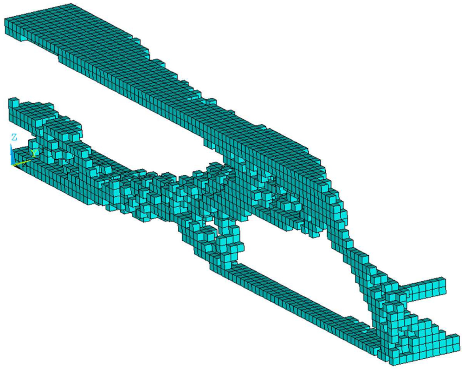
Typical optimal structural topology using 3D BESO.
As has been mentioned, beam–plate structure is often used to provide enough working area; the area of stiffened plate varies from several square meters to several thousand square meters, whereas the thickness is usually millimeter-scale. The elements associated with working area should not be deleted, and the element size should be smaller than or equal to the minimum geometrical feature size, namely, the thickness of stiffened plate, then the scale of whole finite element analysis (FEA) model will be very large; 13 hence, the calculation cost of optimization process will be increased. For example, given the size of a stiffened plate is 20,000 mm × 10,000 mm × 10 mm, the total element number is 2000 × 1000 when the brick element size is set as 10 mm × 10 mm × 10 mm. Not only that, it is hard to change the element size during the optimization process. Usually, it is required to change local plate thickness to inspect the optimization performance according to stress distribution; however, with the brick element design domain, plate thickness change is limited to integral multiple of the default element size; otherwise, the change must include all the elements associated with the plate if much more thickness value is considered, such as 11 and 12.5 mm.
Currently, it is well accepted that lattice structure has better structural performance than its counterpart; therefore, through the above analysis, this article puts forward using shell element to create the basic cell type for generating initial design domain to further improve the performance of 3D BESO for beam–plate structure optimal design.
In the proposed optimization method, a unit cell is used to build the whole design domain, which is the simplest repeating unit. A typical periodic frame of ground structure is shown in Figure 4. The unit cell is represented by areas and points of connection, which are nodes in FEA model. With a certain route of repeating unit cell, the overall frame can be generated first and can be converted to the ground structure based on a given thickness. That being said, the unit cell type plays an imperative role in the proposed optimization method. The data model of the ground structure is shown in Figure 5.

Periodic frame of ground structure.

Data model of ground structure.
As shown in Figure 5, the data model of the ground structure contains four main parts: main dimension parameters, function, material, and periodic frame, which covers optimization levels of shape, topology, and section. For the periodic frame, it can be generated from unit cell type with specified dimensions. In the data structure of shell element, “ID” is used as an index for deleting or adding element. “Plane” is used to describe which plane is the current element associated with and can be used for statistical analysis of element distribution within planes. “Nodes” records nodes data of the current element, while “Edges” is for edges data; these two properties can be used to find neighbor elements. “Equivalent_Stress” is the Von-Mises stress of the current element, which is the most important factor that decides if it should be deleted. The term “is_deleted” indicates the absence/presence state of the current element, while “can_not_delete” is used to indicate if the current element belong to certain working area so cannot be deleted. “Neighbor_Element_IDs” is the set of neighbor element IDs of the current element, which are determined when the periodic frame is set. “Area” and “Center_of_Gravity” are the basic geometrical data of the current element.
Overall process of BESO-based beam–plate structure optimization method
The general flow of this proposed method for beam–plate structure optimization is shown in Figure 6, which consists of two main stages. The first optimization stage is on the topology level, where the optimal topology needs to be found with fixed main dimension parameters. In the second optimization stage, the section parameters are extracted from the rough topology and need to be further optimized using response surface method (RSM). These two optimization stages will be discussed in the following three sections.
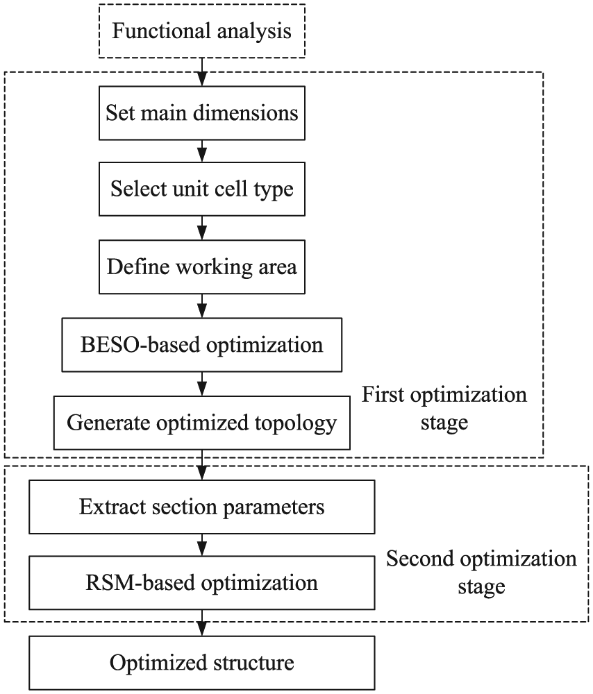
The general flow of the proposed optimization method.
Initial design domain generation
Based on the data model of ground structure, the initial design domain can be generated with specified size and shape parameters. First, the main dimension parameters can be determined based on the functional requirement analysis of the structure. And then, material information should be added. It is suggested to apply same thickness value to each shell element, so that the optimal topology can be revealed under the condition of homogeneity.
Second, the basic unit cell type should be selected, which may further improve the mechanical performance of the designed structure. Figure 7(a) shows three types of basic unit cell where the design domain has cuboid shape or is composed of cuboids. Type 1 is a cubic box. On the basis of type 1, type 2 and type 3 increase web plates with different orientation angles. A simple case has been done and shown in Figure 7(b). In this case, mass, maximum equivalent stress, and strain energy of ground structure with these three types of unit cell have been calculated based on FEA. By comparing the mass, maximum equivalent stress and strain energy of ground structure with these three unit cell types, it is clear that the selection of unit cell type has a significant effect on the mechanical performance of the designed structure. In this step, it is important to set the size of unit cell, which should be smaller than the minimum geometrical feature size. The three dimensions of structure are exact integer multiples of those of unit cell. With smaller the size of unit cell, the more reasonable the optimal result will be achieved, while the calculation scale will be enlarged. The best fit size value of unit cell can be determined by several trial computations with the limitations of hardware.

Comparison of basic unit cells: (a) Three types of basic unit cells and (b) the effect of unit cell type on the structural performance.
Third, the property “can_not_delete” should be set. Elements associated with working area must not be deleted, so the working area should be determined, and then, the elements associated with working area can be recognized. Moreover, by setting the property “can_not_delete” before optimization, the proposed method can be used for optimization of structure in any shape.
BESO-based optimization algorithm
The BESO method is a topology optimization method based on FEA; the basic thought is iteratively removing inefficient material from the designed structure while adding efficient material to the designed structure. BESO is developed from ESO, which was first proposed by Querin et al. to enhance the optimization performance of ESO.
In this article, a modified BESO algorithm is proposed to optimize the shell element distribution for beam–plate structure. The mathematical representation of the proposed BESO problem can be expressed as follows
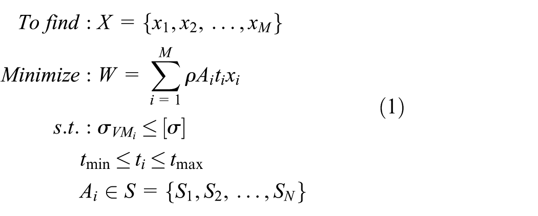
where
Step 1. Set up FEA model. In this model, shell element is used to model the face of the unit cell, and all the shell elements share a same thickness value. All the shell elements are divided into two parts: the elements cannot be deleted and the elements can be deleted. The two parts are denoted as SE1 and SE2, respectively.
Step 2. Recognize all the neighbor elements of each element. For each element e, this function finds out the surrounding elements
Step 3. Apply the boundary conditions, loads.
Step 4. Perform a linear static FEA of the structure.
Step 5. Calculate maximum von Mises stress of each shell element in SE2 and sort them in ascending order. SE2 should be refreshed by excluding the elements already deleted before every iteration step.
Step 6. According to a prescribed rejection ratio

where
Step 7. If the iteration has not been started, it means that the structure is weak, so the thickness should be increased to make sure that the structure has some redundancies, which needs to return to step 1. If the iteration is in progress, it means that some efficient materials have been deleted in last iteration, which should be recovered in this iteration. There are two ways to recover deleted elements. First, a higher initial rejection ratio will cause more elements to be deleted, then need to return to the previous iteration step and lower the rejection ratio, and continue the iteration process. If this method cannot lower the stress, then execute the second method, which is selecting the elements that von Mises stress has exceeded the allowable stress, and recovering the removed neighbor elements. The set of IDs of recovered elements is stored in a list rec_elem_list_i.
Step 8. Repeat steps 3–7 when stop condition is not met.

General workflow of BESO-based optimization algorithm.
There are some rules for the proposed algorithm which are described as follows:
Rule 1. In step 6,
Rule 2. Stop condition includes that del_elem_list_i equals rec_elem_list_i+1, and
Rule 3. To maintain the structure continuity during the process of recovering/deleting elements, if all the neighbor elements of element e are deleted, then element e should also be deleted. This rule is suitable for both “hard-kill” and “soft-kill” strategies.
RSM-based optimization process
Generally, the manufacturability of the optimal topology of BESO method is bad; hence, it is necessary to convert to make the connection part smoother and have a better manufacturability. An example of conversion is given in Figure 9. In Figure 9(a), the blank cell means that the elements are deleted, while the shadowed cells represent the remained elements. It is clear that the remained area has a shape of inclined brace bar, which can be described by four size parameters, as shown in Figure 9(b). The conversion of optimal topology of BESO method will cause many undetermined section parameters based on a relatively fixed topology, which is a complex problem with high computational expense and also a continuous variable optimization problem. An effective and easy method is to use surrogate model to simulate the real problem. Response surface (RS), 14 design and analysis of computer experiments (DACE), 15 and artificial neural network (ANN) 16 are three common approximations usually used to surrogate the original simulation model. In this article, to deal with the complex variable determining problem in large design space, RSM is adopted to reduce computational expense and satisfies the computational precision simultaneously. The second-order model is widely used because of its flexibility and ease of use. With k variables, it can be written as follows

where
Step 1. Confirm the inputs and outputs of section optimization problem. Inputs refer to design variables, while outputs refer to performance.
Step 2. Create the sample points of inputs using Latin hypercube sampling (LHS).
Step 3. Start with
Step 4. Check the model adequacy; if the adequacy is satisfied, then go to step 5; else, go to step 3.
Step 5. Analyze the stationary point to find location of stationary point for the model.
Step 6. Confirm the RSM of section optimization problem.

An example of modification of optimal topology: (a) The irregular layout of remained elements with bad manufacturability and (b) the modified shape of remained area with smoother edges.
Based on the built RS model, the weight optimization problem can be expressed as follows

It is easier to solve this problem using conventional optimization methods, such as sequential linear programming (SLP) algorithm, branch and bound algorithm, and cupidity algorithm.
Case study
Example of cantilever beam design
In this section, an optimization case for a cantilever beam is given to validate the proposed optimization method for beam–plate structure. This part is originally designed with steel, whose material properties are shown in Table 1.
Material properties of steel.

Based on the functional analysis, the main dimensions of cantilever beam are determined as 500 mm × 100 mm × 100 mm. The cantilever beam is clamped at one end and loaded at the center of bottom edge of the opposite tip, which is shown in Figure 10. Based on the design parameters shown in Table 2 and the optimization parameters shown in Table 3, the initial structures are generated and optimized. The problem is symmetric, and thus, only a half domain is modeled.

Cantilever beam design problem.
Design parameters of ground structure.
Value of optimization parameters.

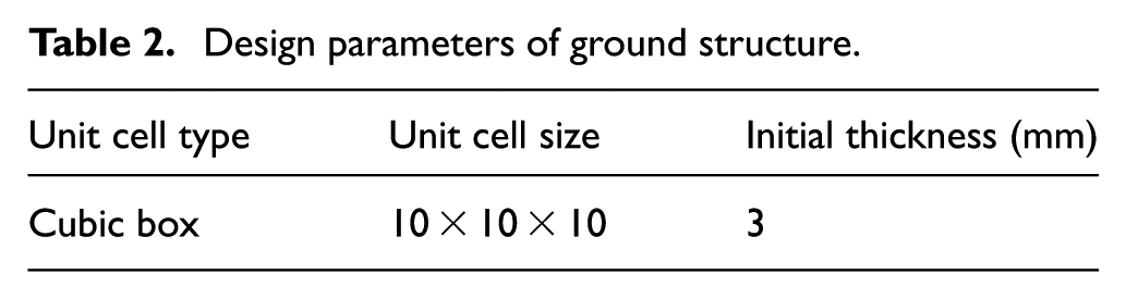
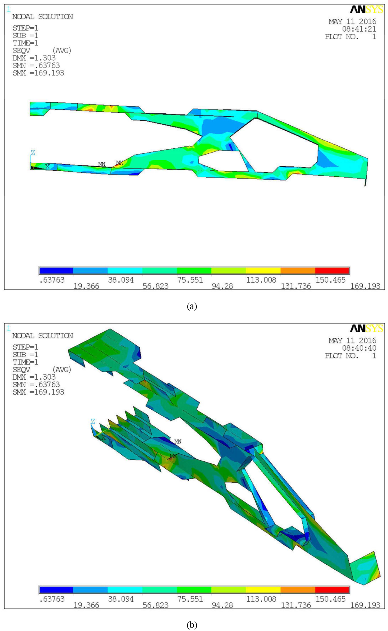
The result of BESO-based optimization is shown in Figure 11. To get better insight into the problem convergence and the contribution of the proposed algorithm, history of the design attributes for the design solutions of the optimization problems is given in Figure 12 with respect to optimization cycle number n.

Result of BESO-based optimization: (a) main frame of optimized topology and (b) overall view of optimized topology.

History of design attributes of BESO-based optimization: iteration history of (a) the ratio of maximum equivalent stress to allowable stress, (b) the ratio of weight to the initial weight, and (c) the rejection ratio.
The optimization process has confirmed the necessity of dynamic rejection ratio. Iteration step 0 in Figure 12 shows the initial stress, weight, and rejection ratio. Note that the curve of rejection ratio has a stairstep shape. Given a fixed rejection ratio, with the optimization process going, the elements must be deleted excessively, and then, the stress will exceed the allowable stress. Assume that there are 10,000 elements in the ground structure, and there will be 200 elements in final solution; if the rejection ratio is kept as 0.2, then in the 18th iteration, there are 225 elements left, and in the 19th iteration there are 180 elements left, which means that 20 elements should not be deleted. As described in the workflow in Figure 8, under this circumstance, the values of present state of all elements are recovered as the previous iteration step, and the rejection ratio is reduced by half to continue the execution of optimization process. With the rejection ratio diminishing gradually, it is indicated that the elements need to be adjusted also reduce, and the distribution of elements will eventually stabilize. As shown in Figure 12(c), in total, 86 iteration steps, the rejection ratio has been reduced six times. Summary on the topology optimization results is given as follows:
Optimal solution is proposed with the mass of 1.2427 kg.
Structural mass is reduced successfully for 18.3283 kg or 6.35% with respect to the initial mass.
Safety is increased by reducing the unnecessary elements.
The computation cost can be thought negligible with respect to the numerous potential solutions.
To express the overall iteration history clearly, the data about stress and weight are processed by normalization. Figure 12(a) shows the iteration history of the ratio of maximum equivalent stress to allowable stress. Figure 12(b) shows the iteration history of the ratio of weight to the initial weight. Figure 12(c) shows the iteration history of the rejection ratio.
The initial rejection ratio is set as 0.2. In the first eight iterations, the weight decreases quickly because there exist redundant elements in initial design domain; however, at the eighth step, the maximum equivalent stress has exceeded the allowable stress which means that some efficient elements are mistakenly deleted. At the ninth step, the mistakenly deleted elements are recovered, and the rejection ratio is lowered as half of the initial value and the iteration is continued. It can be observed from Figure 12(b) that the weight of step 7 is the same as the weight of step 9. These steps demonstrate the necessity of using dynamic rejection ratio; otherwise, the iteration cannot continue. In the following steps, the mechanism is repeated by six times; at last, the rejection ratio has diminished as 0.001625. Figure 12(a) shows that in the last six steps, the maximum equivalent stress has exceeded the allowable stress twice, while the rejection ratio has been lowered twice, and there is almost no change in the weight curve. Actually, the changes are caused by deleting two elements and recovering them. This means that there are no more redundant elements that can be deleted, no matter how small the rejection ratio is. Under this circumstance, the optimization converged for the stop condition is satisfied. Different from some existing methods as genetic algorithm (GA) and ANN, the convergence criterion of proposed method is clear and consistent with the nature of weight optimization problem. Therefore, the convergence in the proposed method can be assured.
Based on the optimal topology, a conversion is carried out. The aim of conversion is to improve the manufacturability, and the conversion is carried out by replacing the jagged edges by straight edges. The main frame is taken as an example to demonstrate how to convert the topology of BESO-based optimization, and Figure 13(a) shows the section parameters of converted main frame. The conversion does not change the topological form and mass distribution, and then, the effect of changes to the current convergence can be ignored. The conversion is about the geometrical shape but not about the element shape. As shown in Figure 13(b), once the geometrical shape is determined, the mesh will be refitted to perform FEA.

Section parameters and mesh change of main frame: (a) section parameters of main frame in conversion and (b) the change of mesh before and after conversion.
To lower calculation cost, the quadratic crossover items in equation (2) are removed, and the RS model is built in the following form

With 236 sampling points, the constructed RS model is expressed as follows

Figure 14 shows the relationship between ×4 and ×6, two of the biggest variables. The 14 section parameters are treated as continuous variables; branch and bound algorithm is adopted to solve the weight optimization problem. Table 4 and Figure 15 show the final optimization result.

Relationship between ×4 and ×6.
Optimal value of section parameters.

Result of RSM-based optimization: (a) main frame of optimized structure and (b) overall view of optimized structure.
The mass of RSM-based optimized structure is further reduced by 2.65%, which is 1.2098 kg. The successful reduction in mass is benefited from the proposed two-stage optimization method. In the first optimization stage, the essence of problem is discrete variable optimization; hence, the optimization result is limited by the fixed size of unit cell, and there is still space for further optimization. Besides that, the conversion of the optimization result from the first stage turned out to be problem of determining the section parameters, which is continuous variable optimization. Clearly, through the second optimization stage, the design parameters of each section can be determined precisely.
In Figure 16, some typical steps in optimization process are selected to demonstrate the mechanism of the proposed method. Figure 16(a) shows the ground structure. Figure 16(b) shows the 8th step where some efficient elements are mistakenly deleted, while Figure 16(c) shows the 10th step where the iteration is continued by lowering rejection ratio. Figure 16(d) and Figure 16(e) show the topology at the 20th and the 40th steps. Figure 16(f) shows the topology of optimal solution in the first stage. Figure 16(g) shows the topology of final optimal solution.

Evolution of topology of optimization results: the topology of (a) ground structure (8300 elements), (b) evolved structure at the 8th step (1710 elements), (c) evolved structure at the 10th step (1928 elements), (d) evolved structure at the 20th step (782 elements), (e) evolved structure at the 40th step (663 elements), (f) optimal solution in the first stage (569 elements), and (g) final optimal solution (the number of elements is not comparable with the above steps).
Comparison of some existing structural optimization methods
To examine the effectiveness and computation efficiency, it is better to compare with existing methods such as traditional BESO and GA. The used parameters and final solutions of three structural optimization methods are listed in Table 5. The mesh size is 10 mm in the three methods. The topologies obtained from these methods are quite different. It is difficult to tell which topology is the best unless the value of objective function is compared. It is observed that the proposed two-stage method produces the lowest value of mass among all the optimization methods, while it takes the smallest number of iterations. Note that the objective function value of BESO with brick element is almost twice as much as the proposed method.
Comparison of some existing structural optimization methods.

BESO: bidirectional evolutionary structure optimization; GA: genetic algorithm.
It should be noted that the BESO method usually requires a finer mesh, especially when the final volume is a low fraction of the initial volume. The computational efficiency of BESO methods highly depends on the parameters including rejection ratio and the mesh size. Usually, a small rejection ratio and a fine mesh can make the optimization process stable and produce a satisfied solution.
Compared to BESO, GA method requires much more iterations and results in the highest value of objective function. In GA method, the amount of computation highly depends on the amount of structural members and the value range of section parameters. The more are the parameters selected, the greater is the amount of computation required. In GA method, the topology of solution of GA is basically the same as the topology of initial solution, whereas the topology of solution of BESO is a little part or even a transformation of the initial solution.
Conclusion
This article presents a two-stage optimization method for beam–plate structure design, which consists of BESO method and RSM. In the first stage, BESO method is used to find the optimal topology. To better fit the beam–plate structure design problem, the initial design domain is composed of box-shaped unit cells, instead of conventional solid units. The optimal topology should be modified to improve the manufacturability; meanwhile, the section design parameters can be extracted for constructing RS model in the second-stage optimization. With an explicit stress function, many existing algorithms can be used to solve the weight optimization problem.
It shows that the solution obtained from the proposed method is noticeably different from those produced by the conventional methods. The results indicate the importance of including topological optimization level and section optimization level in structure design.
In many engineering applications, the design domain is complicated, which may consist of different geometrical shapes, and then, the ground structure cannot be composed of a single type of unit cell. The mixture of different types of unit cells is needed to tackle, but the difficulty becomes a critical consideration. Another consideration is that in BESO method, the topological form of the final solution is limited by the construction of unit cells; hence, the final solution may only be a local optimum. Future research will target at (1) the definition of ground structure when multiple types of unit cells exist and (2) developing more flexible topology evolution strategy that can explore more optimal solutions in a wider range. In addition, it is significant of the way of determining section parameters in the second optimization stage and determining the upper and lower limits of these section parameters; this area is also the subject of the future work.
Footnotes
Academic Editor: ZW Zhong
Declaration of conflicting interests
The author(s) declared no potential conflicts of interest with respect to the research, authorship, and/or publication of this article.
Funding
The author(s) disclosed receipt of the following financial support for the research, authorship, and/or publication of this article: This work was supported by the National-Natural Science Foundation of China (Grant No. 51509033).