The effects of bidirectional evolutionary structural optimization parameters on an industrial designed component for additive manufacture

Abstract

An assessment of the effect of topology optimization design parameters on the performance of an additively manufactured part has been performed. The dependence of the output from a topology optimization involving an aerospace component on the topology optimization control parameters, evolution rate and filter radius was determined. The converged strain energy was found to depend quadratically on the filter radius while the number of iterations required to achieve a solution was broadly related to the evolution rate. These findings demonstrate the potential for significant design efficiencies when manufacturing using additive manufacturing approaches but also the need to be aware of the sensitivity of the bidirectional evolutionary structural optimization optimized design on the selected optimization parameters. This sensitivity can potentially be used advantageously to steer the solution to an optima with features suitable to a particular manufacturing method such as additive manufacturing.

Introduction

Additive manufacture (AM) is a production technique whereby parts are constructed by consolidating successive two-dimensional layers from sliced three-dimensional (3D) models. ¹ It contrasts with traditional manufacturing techniques, which are usually subtractive or formative, and can be used for a range of materials.

These include polymers, ceramics and metals. The layer-by-layer approach has potential economic advantages, since there are few manufacturing constraints and the material required to support the function of a part can, in principle, be minimized. AM does not require tooling, enabling designs with intricate complexities to be built at a reasonable cost. ² It can be argued that complex structures can also be manufactured with processes such as five-axis milling; however, in this case, cost increases significantly with complexity and is restricted by tool access. Also, such subtractive approaches commonly involve processing significantly more material than needed in the final part, causing wastage of both energy and material, with ensuing environmental and cost consequences. ³

Manufacturing processes now being classified as AM include metal deposition (e.g. laser engineered net shaping, direct metal deposition and direct light fabrication), sheet lamination (e.g. laminated object modelling), printing (ballistic particle manufacturing, multijet modelling, 3D printing), powder bed (e.g. selective laser sintering, selective laser melting and electron beam melting), photopolymerization (e.g. solid ground curing and stereolithography (STL)) and extrusion (e.g. fused deposition modelling). ⁴

The level of freedom offered by these processes necessitates the development of new design tools. Current design tools were developed prior to AM and are therefore better suited to traditional manufacturing methods. These tools expedite the design process; however, they can also constrain the complexity of solutions achieved. With traditional manufacturing, this can be advantageous as it can minimize manufacturing difficulties whereas this is not the case for AM. Topology optimization (TO), however, offers even greater potential for AM, since it is capable of achieving complex counter-intuitive solutions. TO is a type of structural optimization that seeks the optimum layout of a design by determining the number of members required in the design and the manner in which these members are connected. ⁵ Algorithms developed for TO include homogenization,^5,6 solid isotropic microstructure with penalization (SIMP)^7–9 and evolutionary structural optimization (ESO).^10,11 Stochastic algorithms used in the broader field of optimization have also been adopted for TO, including genetic algorithms^12,13 and ant colony optimization. ¹⁴ To adopt these algorithms for AM, it is necessary to understand and relax optimization constraints. In a previous study, it has been shown how a shape optimal part can be designed for AM. ¹⁵ In this study, a multidisciplinary approach, incorporating acoustic and modal analysis, was used to optimize the internal and external geometries of a wind instrument.

One promising approach to topologically optimized design for AM is the use of a bidirectional evolutionary structural optimization (BESO).^{10,16,17,18,19} This is a finite element (FE)-based TO method, where inefficient material is iteratively removed from a structure while efficient material is simultaneously added to the structure. BESO is an improvement on ESO that progressively moves a design towards an optimal by removing material from the design iteratively without adding material.^10,11 Querin et al.^10,16,17 implemented an early version of a BESO algorithm in order to enhance the optimization results and speed of the ESO algorithm. Huang and Xie^18,19 presented a modified version of the BESO algorithm that aimed to solve non-convergence and mesh-dependency problems associated with the earlier BESO algorithm. The coupling of this method with AM presents an opportunity for more optimal structures to be realized.

This article investigates the effects of BESO optimization parameters on a relatively simple engineering part currently found in service. Unlike most previous studies, which analysed idealized two-dimensional systems, the part selected demonstrates the potential of TO to achieve large mechanical gains for industrial 3D objects manufacturable via AM. BESO is introduced as an algorithm for minimizing the strain energy, $C$ , of the aerospace part at two volume fraction constraints, $V^{*}$ . Two optimization parameters are varied systematically, and the dependence of $C$ and the number of iterations to convergence on the parameters are investigated.

Solutions from TO normally constitute the first phase of an industrial design process, typically followed by the creation of a computer-aided design (CAD) model and further modifications to ensure structural integrity and manufacturability of the design. While this article concentrates on the TO phase, creation of a CAD model from the TO, validation of the design by experimental testing and analysis and redesign to ensure structural integrity are discussed in sections ‘Experimental validation of topologically optimized designs’ and ‘Structural integrity of topologically optimized design’.

Topology optimization method

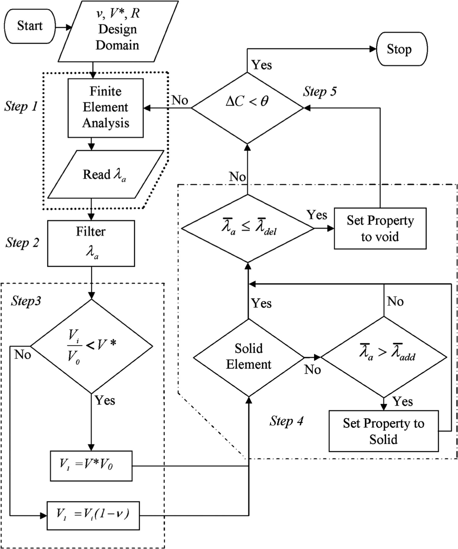
The general methodology is to develop a FE-based model of the system under load and then to couple this to a BESO TO algorithm to seek the optimal design for a given set of conditions. BESO^18,19 requires a number of steps, involving both finite element analysis (FEA), filtering and optimization. In the methodology proposed, the key steps in reaching the optimal solution are as follows:

1. A FEA is performed.

2. The elemental strain energies, ${\lambda }_a$ , read into MATLAB (MathWorks, Natick, MA) and filtered to avoid checkerboarding.

3. A target volume, $V_1$ , is calculated.

4. Elements are classified as either void or solid according to an elemental strain energy threshold, ${\lambda }_{\mathrm{del}}$ .

5. The change in strain energy, $\Delta C$ , over a specific number of iterations is computed and compared to a tolerance, $\theta$ .

6. Steps 1–5 are repeated until $\Delta C$ is lower than $\theta$ .

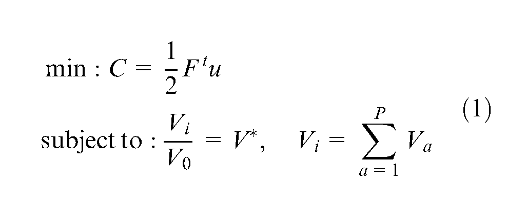
These steps are shown in the flow chart given in Figure 1. For a load, $F$ , causing displacement, $u$ , the problem can be mathematically expressed as

Figure 1.

BESO flow chart to minimize $C$ for a target $V^{*}$ .

$$\begin{array}{c}min:C=\frac{1}{2}{F}^{t}u\hfill \\ \text{subject to}:\frac{V_i}{V_0}=V^{*},V_i=\sum _{a=1}^P{V}_a\hfill \end{array}$$

(1)

where $F^t$ is the transpose of the force vector $F$ ; $V_0$ is the initial volume of a design and $V_i$ is the volume of a design at iteration, $i$ , computed by summing the volume, $V_a$ , of each element, $a$ , at this iteration. $P$ is the total number of elements in a mesh. $V_i$ is divided by $V_0$ to obtain the volume fraction of the design at $i$ . This is iteratively compared to the volume fraction constraint, $V^{*}$ . It should be noted that $V_i=V_0$ at the first iteration.

Two parameters could significantly influence results when this methodology is used to solve a TO problem.^18,19 These are the filter radius, R, and evolution rate, v. This article will focus on understanding the dependence of the solution characteristics on these parameters while solving a $C$ minimization problem for a target $V^{*}$ . The evolution rate, v, is the fraction number used to compute a target volume $V_1$ at i. R is the radius of a sphere sharing its centre with an element, a. Sensitivities of nodes within this sphere are used to calculate filtered elemental sensitivities, $\overline{{\lambda }_a}$ , as will be described later in this section. This step eliminates the occurrence of undesired checkerboard patterns in optima.^5,20–22

The $v$ , $R$ and $V^{*}$ parameters are systematically varied in this study via a series of experiments to determine their effect on the performance and appearance of the resulting topologies.

FEA

The FEA was performed using the commercial FE software, MSC Nastran (MSC Software, California, Santa Ana). The results were passed to a script in MATLAB to perform the TO. Sub-steps within step 1 are shown within the dotted lines in the flow chart (Figure 1).

Filtering elemental strain energies

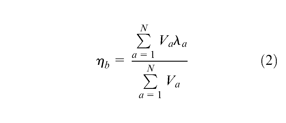
Results from an FEA were passed to a script in MATLAB to perform the TO. Sub-steps within step 1 are shown within the dotted lines in the flow chart (Figure 1). The elemental sensitivities, ${\lambda }_a$ , are equivalent to the elemental strain energies. These elemental strain energies are filtered in two stages. First, a volume weighting of the sensitivities of the elements connected to a node, $b$ , is computed through

$${\eta }_b=\frac{\sum _{a=1}^N{V}_a{\lambda }_a}{\sum _{a=1}^N{V}_a}$$

(2)

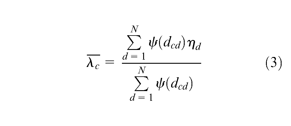
where $N$ is the total number of elements connected to node $b$ . This calculates the average elemental sensitivities associated with the nodes. Second, a longer wavelength elemental sensitivity, ${\overline{\lambda }}_c$ , is calculated by finding nodes $d$ whose distance $r$ to the centre of an element $c$ is less than or equal to the filter radius, $R$ (i.e. $r(c)\le R$ ). These nodes contribute to ${\overline{\lambda }}_c$ according to

$$\overline{{\lambda }_c}=\frac{\sum _{d=1}^N\psi \left(d_{\mathrm{cd}}\right){\eta }_d}{\sum _{d=1}^N\psi \left(d_{\mathrm{cd}}\right)}$$

(3)

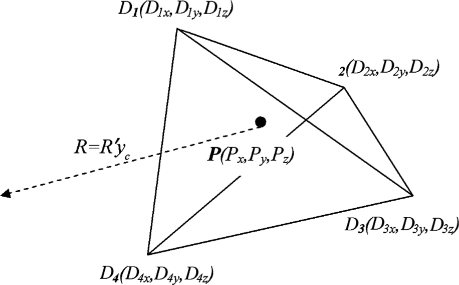
where $\psi (d_{\mathrm{cd}})=R-d_{\mathrm{cd}}$ and $d_{\mathrm{cd}}$ are the distance between node $d$ and the centre of element $c$ . We define $R$ as a multiple of the root mean square distance between the centre P of element $c$ and the nodes D (Figure 2), $y_c$ such that

Figure 2.

Determination of $R$ for a tetrahedral element.

$$R=R\prime y_c$$

(4)

where $R\prime$ is a user-defined scaling factor.

The coordinates of $P$ are calculated by determining the centre of mass

$$P_j=\frac{1}{g}\sum _{d=1}^g{D}_{\mathrm{dj}}$$

(5)

where $j$ is the coordinate direction (x, y, z) and $g$ is the number of nodes for the element. The distance $y_c$ is given by

$$y_c=\sqrt{\sum _{j=x,y,z}{(D_{\mathrm{dj}}-P_j)}^2}$$

(6)

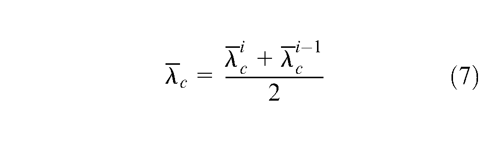
A further step is performed to smooth the filtered sensitivities. The final sensitivity is then given by an average of the current sensitivity, ${\overline{\lambda }}_c^i$ , and the sensitivity at the previous iteration, ${\overline{\lambda }}_c^{i-1}$ , such that

$${\overline{\lambda }}_c=\frac{{\overline{\lambda }}_c^i+{\overline{\lambda }}_c^{i-1}}{2}$$

(7)

${\overline{\lambda }}_c$ is used in step 4 to classify elements as either solid or void.

Computing the target volume

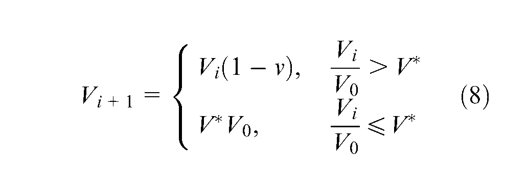
The volume fraction ( $V_i/V_0$ ) of the design is checked iteratively against $V^{*}$ . At each step, if it is greater than $V^{*}$ , then a new target volume, $V_{i+1}$ , is computed from

$$V_{i+1}=\{\begin{array}{cc}\hfill V_i(1-v),\hfill & \frac{V_i}{V_0}>V^{*}\hfill \\ \multicolumn{1}{c}{V^{*}{V}_0,}& \frac{V_i}{V_0}\le V^{*}\hfill \end{array}$$

(8)

such that upon the next iteration, the elements removed bring the volume of the design to $V_{i+1}$ and the design progressively moves towards $V^{*}$ . If the volume fraction of the design reaches a value less than $V^{*}$ , then we compute $V_{i+1}$ from the product of $V^{*}$ and $V_0$ . Sub-steps within step 3 are shown within the dashed line in the flow chart (Figure 1).

Adding and deleting elements

After $V_{i+1}$ is computed, all elements are ranked in descending order of ${\overline{\lambda }}_c$ . The first listed elements, whose total volume equals $V_{i+1}$ , are marked for retention. Therefore, ${\overline{\lambda }}_c$ of the last element in this list is labelled as ${\overline{\lambda }}_{\mathrm{del}}$ . Solid elements having sensitivity values below ${\overline{\lambda }}_{\mathrm{del}}$ are then marked for deletion from the design domain. Deletion is achieved by assigning the element to a void property as the TO progresses, where this void property is defined as having a significantly reduced stiffness to that of a solid element. Young’s modulus of void elements in this case was defined as $1.35\times {10}^{-4}$ times that of solid elements, $E_s$ . Modelling the voids in this way eliminates the need for iterative connectivity checks associated with the total deletion of void elements from the design domain and offers a way to conveniently reincorporate void elements into the design at a later iteration if required. The factor $1.35\times {10}^{-4}$ used to calculate $E_s$ is an empirically determined figure that gave a balance between ensuring a sufficiently reduced stiffness to the void elements for solution accuracy while avoiding excessive ill conditioning in the global stiffness matrix.

An additional group of elements is added to the two defined above. These elements belong to the regions of the domain that are kept solid throughout the optimization, and they model parts in the structure where material should not be removed. Elements belonging to this group are called non-design domain elements while other solid elements are called design domain elements. Non-design domain elements are ignored during the BESO optimization but are included in every FEA iteration. This effect is achieved by defining a unique property identification number for each set of elements in the Nastran input file. The BESO algorithm only uses elements not associated with the non-design property in the TO. Void elements with sensitivities above the threshold, ${\lambda }_{\mathrm{add}}$ , are reclassified as solid elements, bringing the volume of solid elements at $i$ to $V_1$ . This step is skipped at the first iteration since the TO starts from a fully solid design domain.

Convergence check

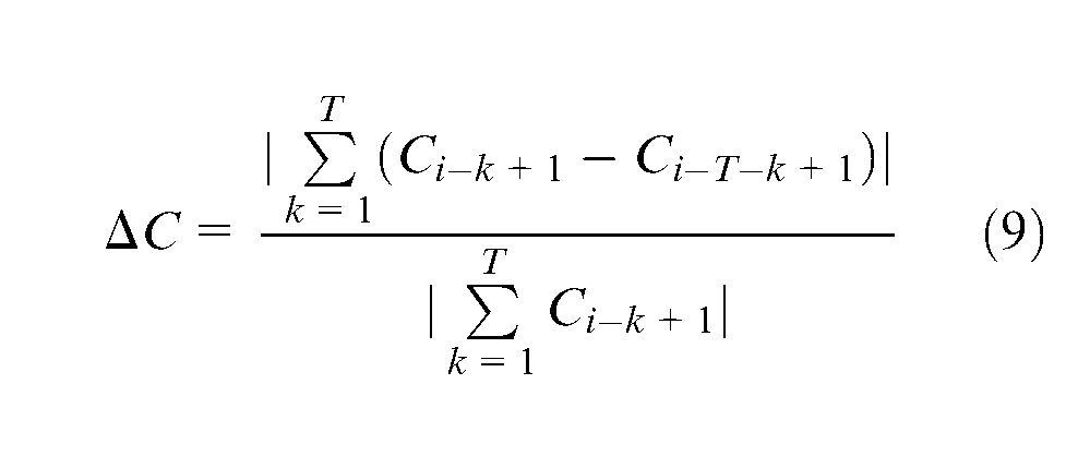
The TO cycle is then repeated until $\Delta C$ is less than $\theta$ , and $V^{*}$ is obtained. We set $\theta$ to ${10}^{-4}$ and the maximum number of iterations to convergence, $i_c$ , to 120 and 400 for high and low $v$ , respectively. This limit is set to avoid becoming trapped within an infinite loop. The variation in selected $i_c$ is because a higher value of $v$ is expected to result in faster convergence than a lower $v$ . $\Delta C$ is computed using

$$\Delta C=\frac{|\sum _{k=1}^T(C_{i-k+1}-C_{i-T-k+1})|}{|\sum _{k=1}^T{C}_{i-k+1}|}$$

(9)

where T = 5, and $k$ is the sequence of integers from 1 to $T$ .

Description of test case

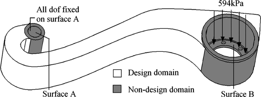
To test this approach to optimization for AM parts, the BESO algorithm was used to solve a 3D TO problem of an aerospace metallic cantilever arm (Figure 3). This object represents a practical problem that will illustrate the capacities and dependencies of the described TO algorithm. Two new levels of difficulty exist for this problem when compared against the two-dimensional or 3D cantilever problems often solved in the literature. These are the existence of a non-design domain and an increased geometrical complexity. The arm is subjected to a single load case, fixing all the degrees of freedom at surface A and subjecting surface B to a pressure of 594 kPa, thereby forming a cantilever beam. The grey portion in Figure 3 is set as the non-design domain while the rest of the domain is classified as the design domain. The objective was to minimize the strain energy of the design domain for a given $V^{*}$ . The material used has a Young’s modulus of $74\text{GPa}$ and a Poisson’s ratio of 0.33.

Figure 3.

Test problem illustrating design domain, load and boundary constraints.

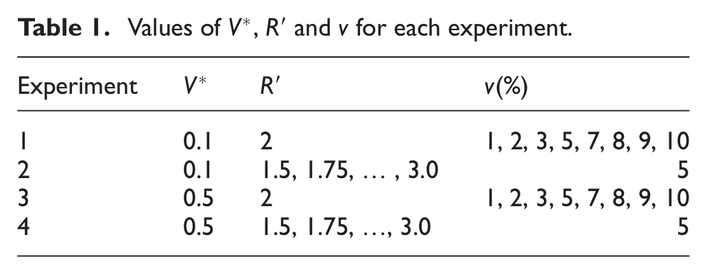
The entire domain was meshed with approximately 300,000 linear tetrahedral unstructured elements, with element volumes approximately equal. Four sets of experiments were performed to investigate the effect of changing $v$ or $R$ on the optima (Table 1).

Table 1.

Values of $V^{*}$ , $R\prime$ and $v$ for each experiment.

Experiment	$V^{*}$	$R\prime$	$v(\%)$
1	0.1	2	1, 2, 3, 5, 7, 8, 9, 10
2	0.1	1.5, 1.75, … , 3.0	5
3	0.5	2	1, 2, 3, 5, 7, 8, 9, 10
4	0.5	1.5, 1.75, …, 3.0	5

To elucidate the behaviour changes for different $V^{*}$ , in the first two sets, $V^{*}$ was set at 0.1, while in the last two sets, $V^{*}$ was set at 0.5. For the first experiment, we kept $R\prime$ at 2 while varying $v$ from 1% to 10%. The dependence of the results on $R\prime$ was then tested by fixing $v$ and varying $R\prime$ from 1.5 to 3 in the second experiment, a range originally proposed by Huang and Xie. ¹⁸ The third and fourth experiments repeated the pattern but with $V^{*}=0.5$ . In addition to the parametric settings in Experiments 2 and 4, the filtering step in the BESO algorithm was skipped for these two experiments to generate unfiltered topologies at both $V^{*}$ . This was done to understand the effects of filtering on the TO results. After the TO, solid elements were extracted from the mesh to define the optima. Also, all elements in the domain were initially associated with the solid Young’s modulus. The strain energy, $C$ ; optimum topologies; iterations at which $C$ peaks, $i_p$ ; iterations at which $C$ converges, $i_c$ and number of members, $M$ , in optima at the two volume fraction constraints were monitored to understand the dependence of the solutions on $v$ and $R\prime$ .

Topology optimization results

Experiment 1

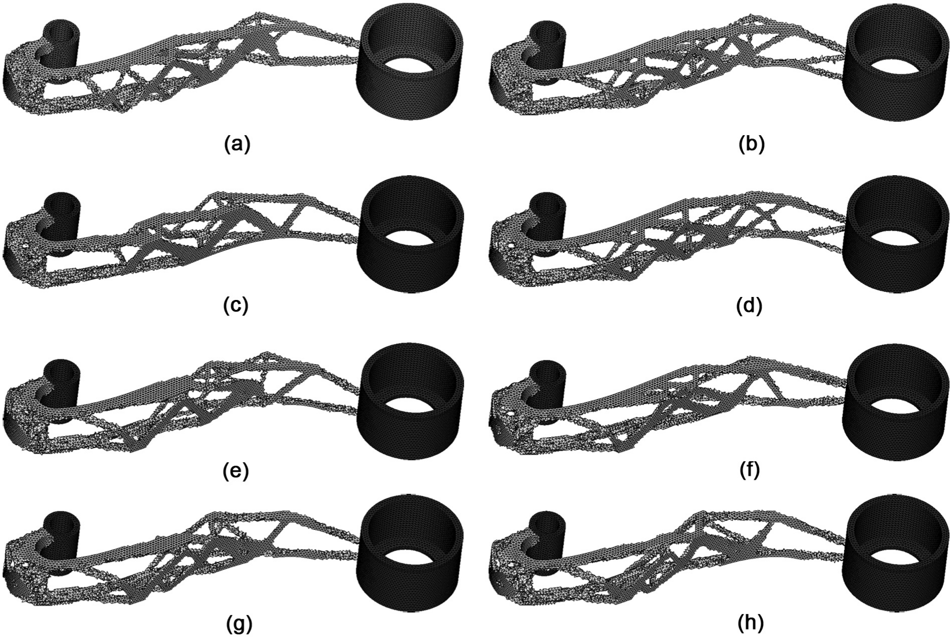
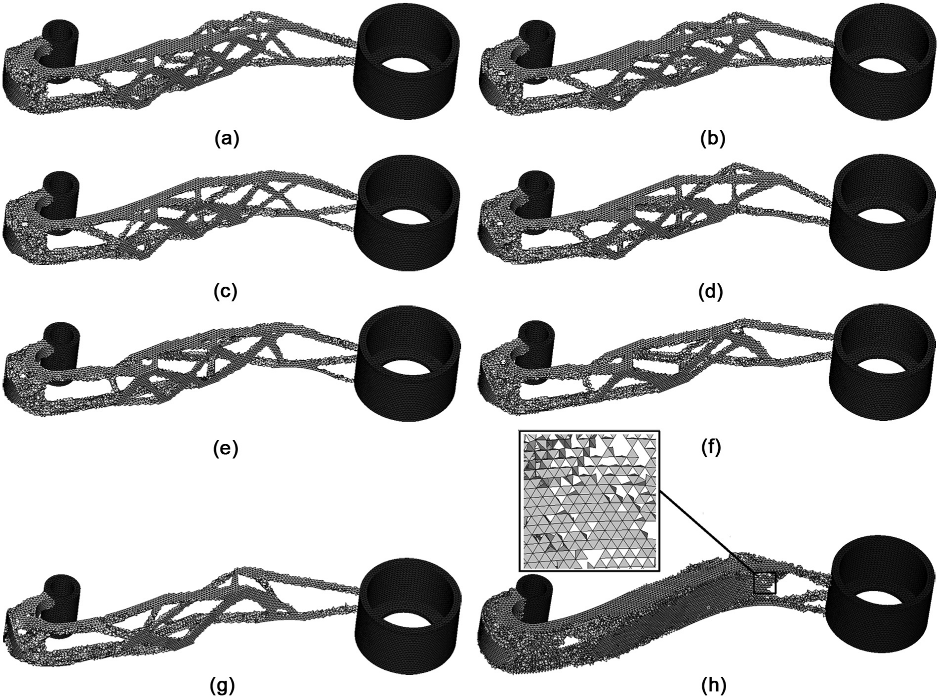
The optimal topologies for the first experiment in which $R\prime$ is fixed at 2 and $v$ is varied are shown in Figure 4. The dependence of the solution on the optimization parameters can be visualized by plotting $C$ against $i$ for all $v$ (Figure 5).

Figure 4.

Different truss-like optimum topologies for Experiment 1 where $v$ is (a) 1%, (b) 2%, (c) 3%, (d) 5%, (e) 7%, (f) 8%, (g) 9% and (h) 10%.

Figure 5.

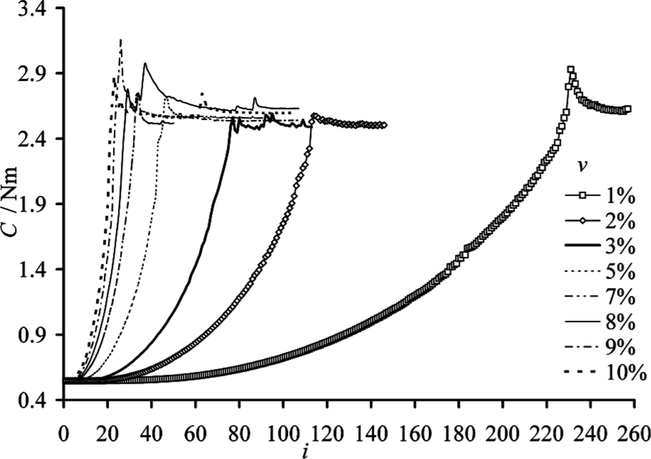
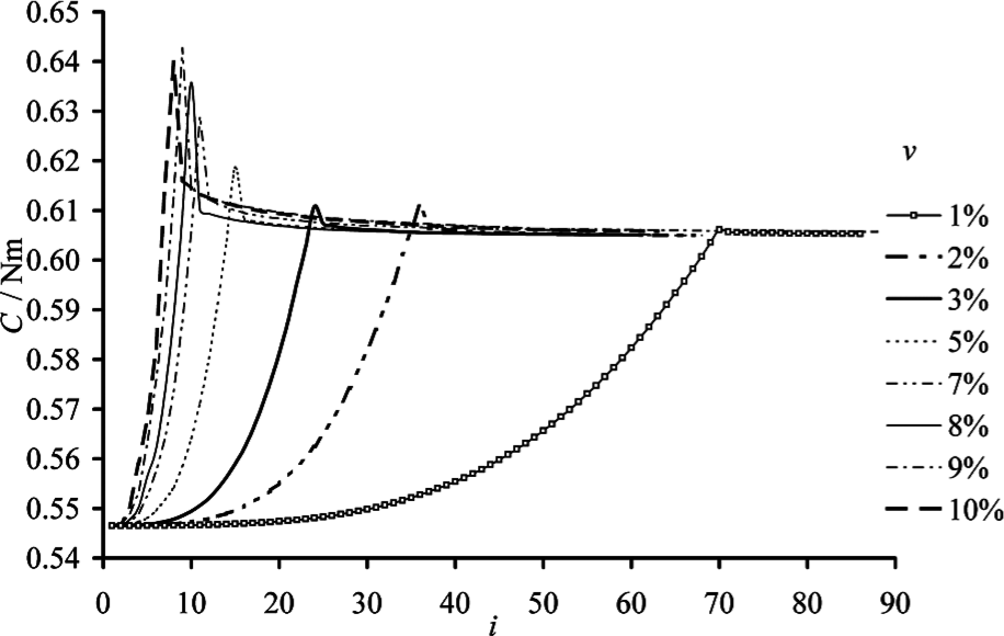
$C$ against $i$ for different values of $v$ at $R\prime =2$ and $V^{*}=0.1$ showing different $C$ profiles.

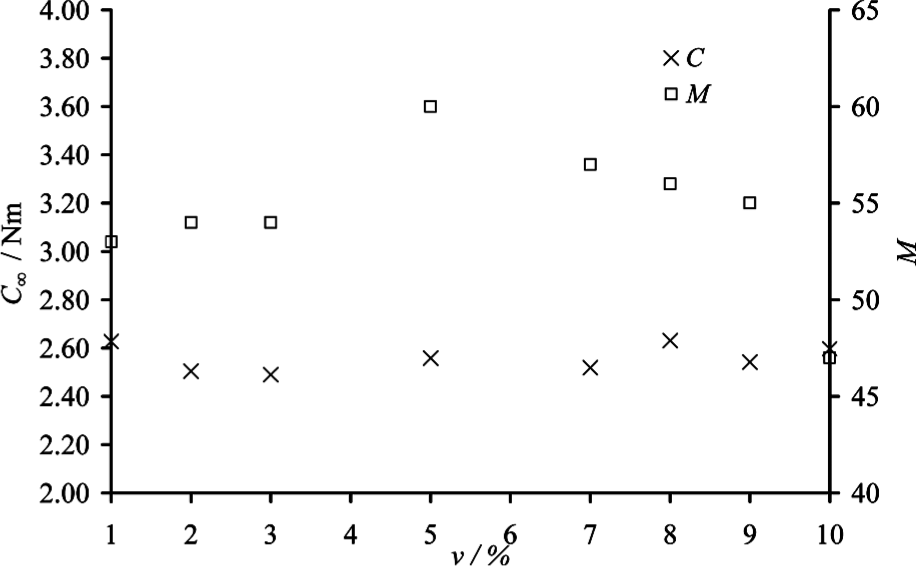
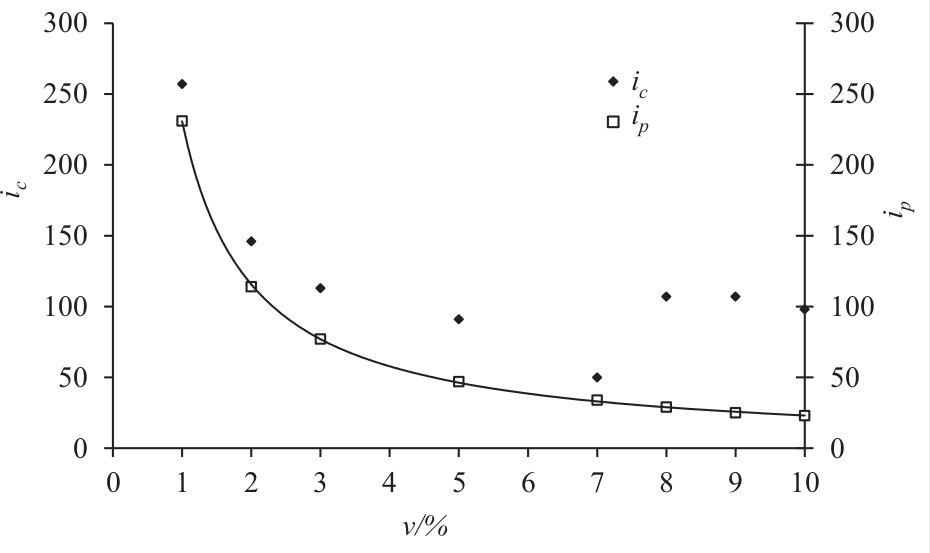
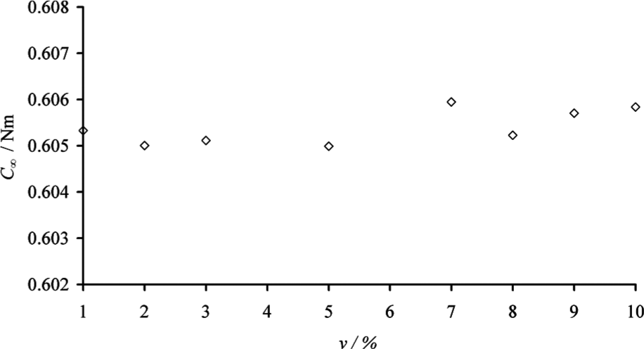
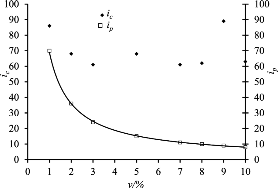
The behaviour of $C$ is characterized by two stages: a monotonic increase in its value up to the point where $V^{*}$ is reached and then a decay in $C$ to an asymptotic value, $C_{\infty }$ . The number of iterations to the peak in $C$ is termed as $i_p$ , and the number of iterations to convergence is termed as $i_c$ . Figure 6 shows the dependence of $C_{\infty }$ and the number of members, $M$ , on $v$ and we see that the final strain energy is relatively insensitive to $v$ . The number of members, $M$ , shows some dependence on $v$ , but the relationship is not clear. The $i_p$ decreases as $v$ increases, as shown in Figure 7, where $i_p$ and $i_c$ are plotted against $v$ . $i_c$ tends to decrease as $v\%$ increases; however, in this case, there appears to be some scatter in the data.

Figure 6.

Behaviour of $C_{\infty }$ and $M$ when $v$ is varied at $R\prime =2$ and $V^{*}=0.1$ .

Figure 7.

$i_p$ and $i_c$ against $v$ at $R\prime =2$ and $V^{*}=0.1$ , where $i_p$ decreases as $v$ increases according to equation (10).

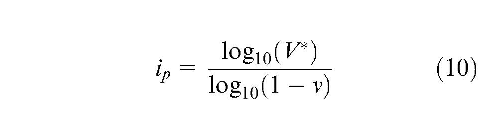
Mathematically, the progressive decrease in $i_p$ obeys

$$i_p=\frac{{\log }_{10}\left(V^{*}\right)}{{\log }_{10}(1-v)}$$

(10)

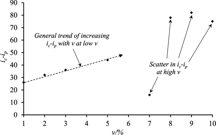
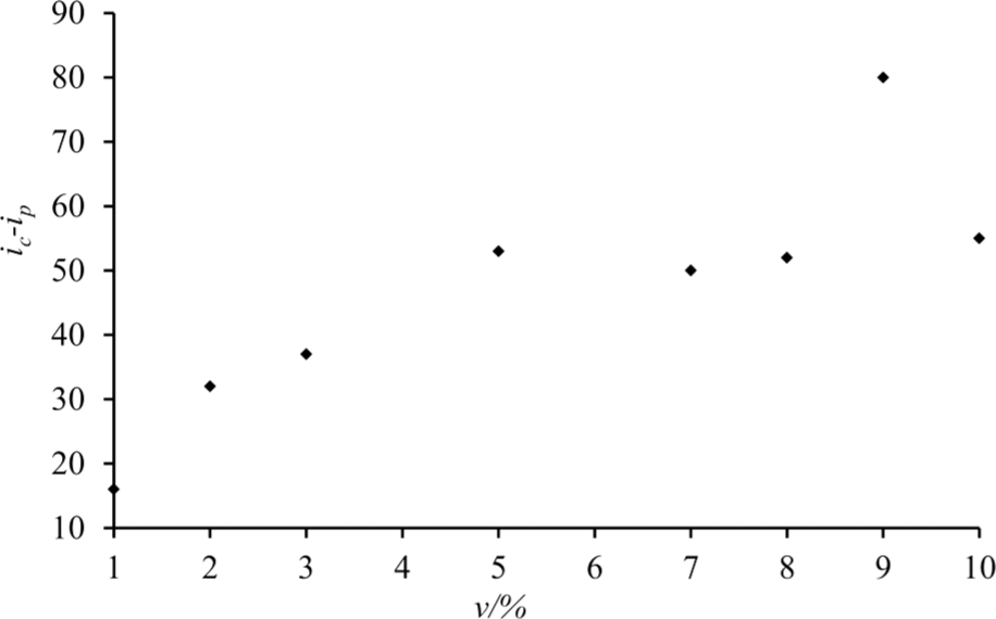
Equation 10 has an $R^2$ value of 1 when fitted to $i_p$ data. Since $i_p$ is controlled by $v$ (equation (8)), this behaviour is expected. Beyond $i_p$ , $V_{i+1}$ is independent of $v$ , where it remains fixed at $V^{*}\times V_0$ (section ‘Description of test case’). The number of iterations in the second stage of the optimization, after the target volume has been reached, is $i_c-i_p$ . A plot of $i_c-i_p$ against $v$ (Figure 8) shows that $i_c-i_p$ increases with increasing $v$ at low values of $v$ but exhibits a high degree of scatter at higher values of $v$ . This is understandable as the first stage of the TO, where C increase involves both element removal and stress redistribution. Therefore, a greater number of iterations to reach the peak value of $C$ at low $v$ would allow the solution to achieve a closer to optimal topology, and a smaller number of iterations would be expected in the second stage of the optimization. However, at very high $v$ , the combination of few iterations and large volume removed at each iteration leads to scatter in the plot of $i_c-i_p$ against $v$ . As $i_c$ is dominated by the first stage of the TO (i.e. by $i_p$ ) at low $v$ , it can be seen in Figure 7 that the plot of $i_c$ against $v$ follows a similar trend to $i_p$ against $v$ . However, at high $v$ , the second stage of the TO (i.e. $i_c-i_p$ ) becomes more dominant, resulting in a divergence of the plot of $i_c$ against $v$ from the line of $i_p$ against $v$ and appearance of the scatter in the value of $i_c-i_p$ at high $v$ .

Figure 8.

$i_c-i_p$ against $v$ at $R\prime =2$ , $i_c-i_p$ is observed to increase as $v$ is increased, peaking at $v=9\%$ .

Experiment 2

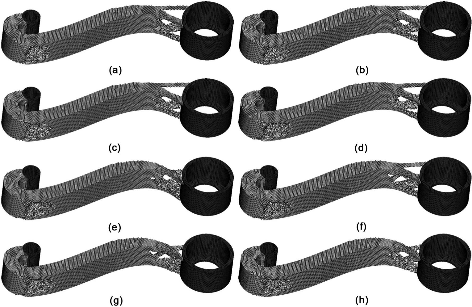
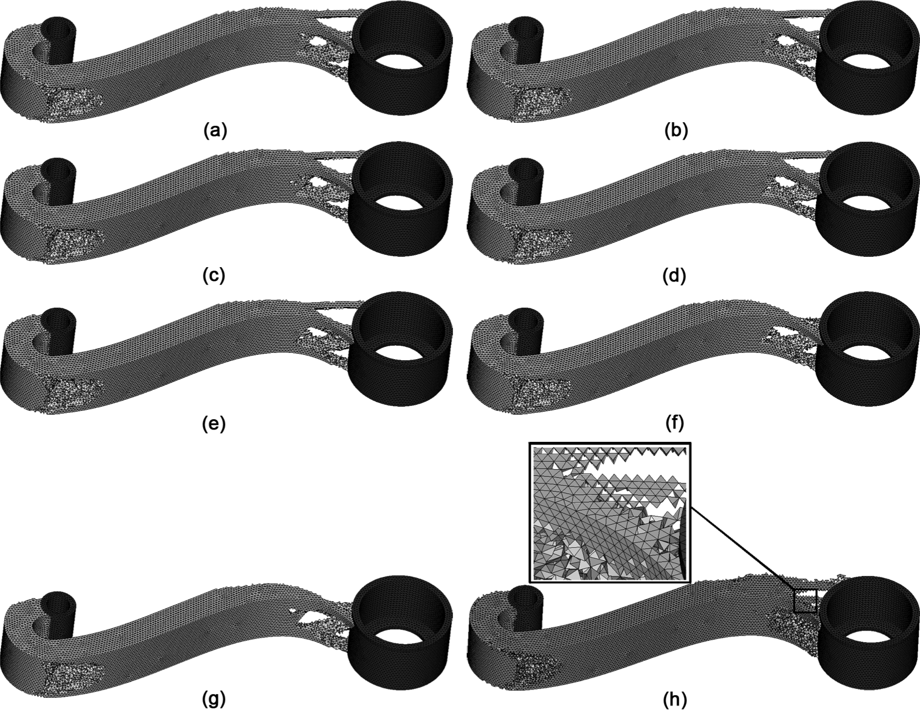
The dependence of optimal topologies on $R\prime$ for a target volume $V^{*}=0.1$ was explored in Experiment 2. Figure 9(a) to (g) shows the topologies achieved by filtering ${\lambda }_a$ for the different values of $R\prime$ , while Figure 9(h) shows the topology when filtering is not used. Inspection of the solutions shows that there is not any checkerboard pattern after filtering, but it is evident in the unfiltered case. As expected, the solutions are similar to those observed in Experiment 1 (Figure 4).

Figure 9.

Different truss-like optimal topologies for Experiment 2 where $R\prime$ is (a) 1.5, (b) 1.75, (c) 2.0, (d) 2.25, (e) 2.5, (f) 2.75, (g) 3.0 and (h) unfiltered with checkerboarding.

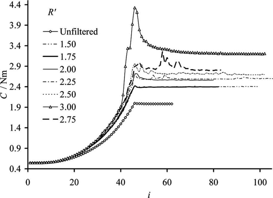
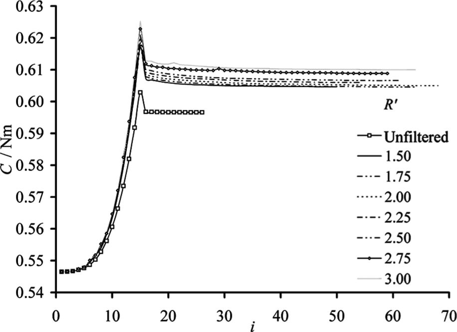
The value of the strain energy as the optimization proceeds is shown in Figure 10. Both $i_p$ and $i_c$ were found to be largely independent of $R\prime$ , although some variation was seen in the value of $i_c$ . The peaks in $C$ tend to occur after broadly the same number of iterations ( $i_p\approx 46$ ), regardless of the value of $R\prime$ , suggesting that for this target volume, $i_p$ is independent of $R\prime$ as we would expect. After $i_p$ , solutions converge to a different $C_{\infty }$ , the value of which is dependent on $R\prime$ .

Figure 10.

$C$ against $i$ for different values of $R\prime$ at $v=5\%$ and $V^{*}=0.1$ showing different $C$ profiles.

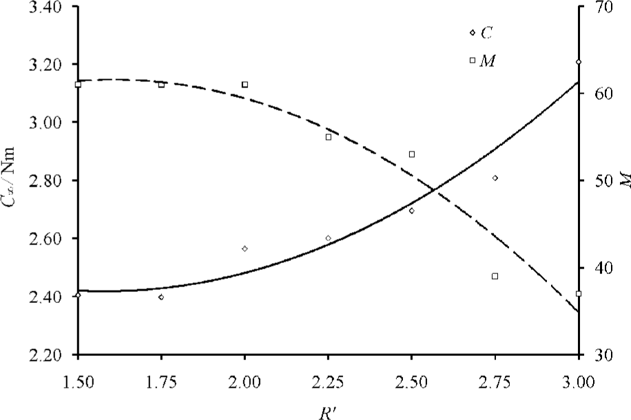
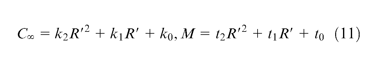
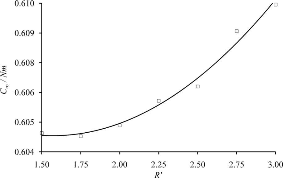
It is worth noting that it appears as if the topology reached without filtering (Figure 9(h)) has a lower $C_{\infty }$ than the other solutions, suggesting that this may be the best result. A second look, however, shows that it cannot be compared easily with the other topologies (Figure 9(a) to (g)) since checkerboard patterns within this topology make it ultimately suboptimal. The dependence of $C_{\infty }$ and $M$ on $R\prime$ is shown in Figure 11. The final strain energy, $C_{\infty }$ , increases with $R\prime$ , while the number of members, $M$ , reduces with increasing $R\prime$ . This latter effect can be understood in terms of the filter radius, $R\prime$ , smoothing out short wavelength features, thereby reducing the number of members. $C_{\infty }$ and $M$ relationships with $R\prime$ were quantified with a second-order regression (solid and dashed line in Figure 11), such that

Figure 11.

$C_{\infty }$ and $M$ against $R\prime$ , $C_{\infty }$ increases and $M$ decreases as $R\prime$ is increased. A second-order regression is fitted to both data sets.

$$C_{\infty }=k_2{R\prime }^2+k_{1}R\prime +k_0,M=t_2{R\prime }^2+t_{1}R\prime +t_0$$

(11)

where $k_2$ , $k_1$ , $k_0$ , $t_2$ , $t_1$ and $t_0$ are constants that depend on the geometry and target volume. For Experiment 2, $k_2$ , $k_1$ and $k_0$ were determined to be $0.36$ , $-1.13$ and $3.31$ , respectively (solid line in Figure 11) with $R^2=0.95$ ; $t_2$ , $t_1$ and $t_0$ were found to be $-18.95$ , $68.02$ and $0$ , respectively (dashed line in Figure 11) with $R^2=0.93$ .

Experiment 3

It was anticipated that changing $V^{*}$ would affect the TO. To investigate this, $V^{*}$ was increased from 0.1 to 0.5 and Experiment 1 repeated. The solutions are shown in Figure 12. Clear differences can be seen between the topologies here and those when $V^{*}=0.1$ (Figures 4 and 9). In particular, a common feature of these topologies is the hollow shell in the design domain not found in the previous truss-like topologies (cf. Figures 4 and 9).

Figure 12.

Optimum topologies for Experiment 3 where $v$ is (a) 1%, (b) 2%, (c) 3%, (d) 5%, (e) 7%, (f) 8%, (g) 9% and (h) 10%.

The development of the strain energy during the experiment is shown in Figure 13, and it can be seen that $C_{\infty }$ are lower than those observed in Experiment 1. This is attributable to the object deflecting less since more material exists in the optima at this $V^{*}$ . As was the case for Experiment 1, $C_{\infty }$ is independent of $v$ (Figure 14). In Figure 15, $i_p$ and $i_c$ are plotted against $v$ , showing that $i_p$ decreases as $v$ is increased. Similar to Experiment 1, this behaviour can be represented by equation (10) with an $R^2$ value of 1.

Figure 13.

$C$ against $i$ for different values of $v$ at $R\prime =2$ and $V^{*}=0.5$ , curves having different peaks but approximately same $C_{\infty }$ .

Figure 14.

$C_{\infty }$ against $v$ at $R\prime =2$ and $V^{*}=0.5$ showing $C_{\infty }$ is insensitive to $v$ .

Figure 15.

$i_p$ and $i_c$ against $v$ at $R\prime =2$ and $V^{*}=0.5$ , where $i_p$ decreases as $v$ increases according to a power equation.

Again, a plot of $i_c-i_p$ against $v$ (Figure 16) suggests an increase in $i_c-i_p$ as $v$ is increased, at low values of $v$ , with more random behaviour at high $v$ . In Figure 15, it can be seen that there is a steady decrease in $i_c$ at low $v$ , where $i_p$ dominates, with significant scatter at high $v$ , where contributions from $i_c-i_p$ to $i_c$ become significant.

Figure 16.

$i_c-i_p$ against $v$ at $R\prime =2$ , $V^{*}=0.5$ ; $i_c-i_p$ is observed to increase as $v$ is increased, peaking at $v=9\%$ .

Experiment 4

In Experiment 4, the dependence on $R\prime$ is determined for a target fraction, $V^{*}$ , of 0.5. The solutions obtained are shown in Figure 17 and show small variations, but with a consistent hollow shell topology. No checkerboard patterns were found in the filtered solutions (Figure 17(a) to (g)) but were significant in the unfiltered solution (Figure 17(h)).

Figure 17.

Similar optimal topologies for Experiment 4 where $R\prime$ is (a) 1.5, (b) 1.75, (c) 2.0, (d) 2.25, (e) 2.5, (e) 2.75, (g) 3.0 and (h) unfiltered with checkerboarding.

The peak strain energy is seen to occur at the same $i_p$ for all $R\prime$ (Figure 18). Again, it is observed that the filter radius has little effect on $i_p$ or $i_c$ , although a slow rate of convergence to $i_c$ is seen for the unfiltered solution. This suggests once more that the rate at which a solution is obtained is independent of the degree of filtering performed. Conversely, when the final strain energy, $C_{\infty }$ , is plotted against $R\prime$ , a strong relationship is observed that is reasonably well represented by equation (11). A second-order regression of equation (11) was fitted to the experimental data, where the values of $k_2$ , $k_1$ and $k_0$ were $0.0027$ , $-0.0086$ and $0.6113$ , respectively, with $R^2=0.98$ (solid line in Figure 19).

Figure 18.

$C$ against $i$ at different $R\prime$ where $v=5\%$ and $V^{*}=0.5$ , curves having same $i_c$ but different $C_{\infty }$ .

Figure 19.

$C_{\infty }$ against $R\prime$ at $v=5\%$ and $V^{*}=0.5$ fitted with a second-order regression showing $C_{\infty }$ is strongly dependent on $R\prime$ .

BESO parameter relationships

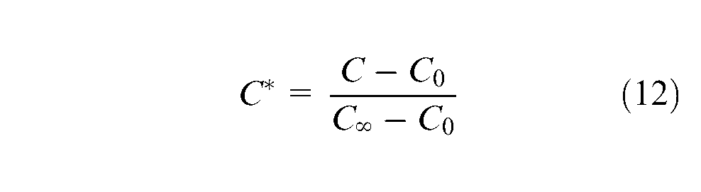
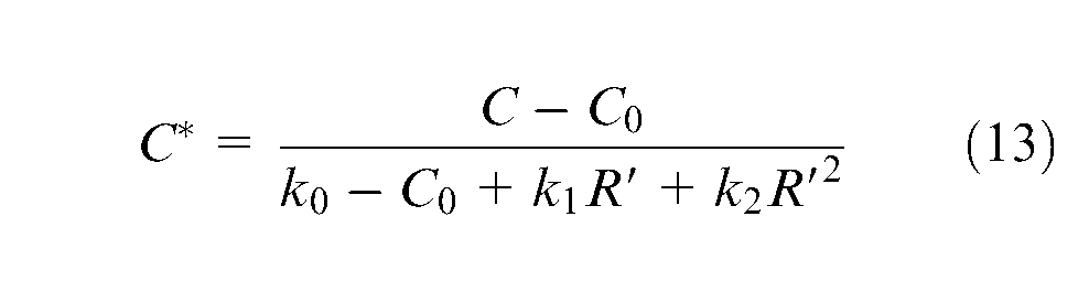
The results for $V^{*}=0.1$ and $V^{*}=0.5$ demonstrate that there are underlying trends in the performance of the BESO algorithm that can be used to tune its efficiency and efficacy. These results indicate that the rate at which a solution is achieved is controlled by $\mathrm{iv}$ . In addition, the quadratic relationship between the asymptotic strain energy and $R\prime$ suggests that it is possible to determine a curve that represents the characteristic behaviour of the TO within the parametric domain studied. Examining Figures 10 and 18, it can be seen that it is possible to determine a new variable, $C^{*}$ , that is given by

$$C^{*}=\frac{C-C_0}{C_{\infty }-C_0}$$

(12)

where $C_0$ is the strain energy at $i=1$ . Since it is possible to determine the relation between $C_{\infty }$ and $R\prime$ through equation (10), equation (11) becomes

$$C^{*}=\frac{C-C_0}{k_0-C_0+k_{1}R\prime +k_2{R\prime }^2}$$

(13)

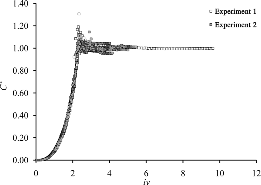
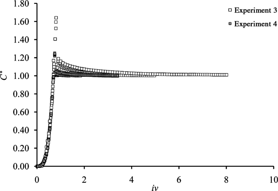
where $k_0$ , $k_1$ and $k_2$ depend on the target volume $V^{*}$ . Figures 20 and 21 show the scaled variables for both target fractions. It can be seen that the curves tend to fall on to two master curves, the difference between Figures 20 and 21 illustrating the greater number of iterations that need to be made before a solution is found for $V^{*}=0.1$ than for $V^{*}=0.5$ .

Figure 20.

General behaviour of scaled data from Experiments 1 to 4 where $V^{*}=0.1$ .

Figure 21.

General behaviour of scaled data from Experiments 5 to 8 where $V^{*}=0.5$ .

The curves demonstrate the consistent behaviour of the algorithm in the chosen parametric domain. The dependence on $R\prime$ is expected since the filtering process will act as a low-pass filter and smooth the topology, changing the characteristics in a controlled and continuous fashion.

Comparison with SIMP

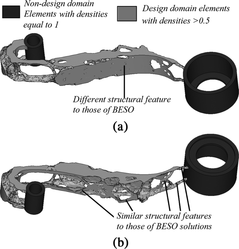
Most commercial TO software currently uses the SIMP method, which contrasts with the BESO method by utilizing element density (usually equated to stiffness) as the design variable and introducing a penalty on intermediate densities to drive a solution towards a void–solid representation. ⁷ In most cases, some intermediate densities remain in the final solution, and these can be removed by thresholding at a user-defined density to make the structure manufacturable. A completely fair comparison of the performance of the BESO and SIMP algorithms is not possible because of the fundamentally different processes involved and the dependence of each on their optimization parameters; however, to illustrate the two methods, a commercial software (OptiStruct, Altair Engineering, Troy, MI, USA) based on the SIMP algorithm was used to obtain a TO structure for the test case with $V^{*}$ of 0.1, using comparable material properties and initial mesh to that used in the BESO studies but with an initial elemental density of 0.9. The main parameter used in the SIMP algorithm is the penalization factor, which was set to 1.5 in this case. This value was chosen to be greater than one to suppress, to a large extent, the appearance of intermediate densities but low enough to prevent a local optima. The optimal solution from the SIMP TO, with element thresholding at a density of 0.5, is shown in Figure 22.

Figure 22.

Solution achieved from a SIMP-based software: (a) front view and (b) rear view.

It can be seen that many of the features are similar to those seen in the BESO solutions; however, the solid skins seen at the boundaries of the design domain appear to be a feature of the evolution of the final solid–void structure from one of variable density. This solution had a $V^{*}$ of 0.1 and $C_{\infty }$ of 4.43 Nm, which is higher than that seen in the BESO solutions. This single test case cannot be used to make any general assumptions about the performance of the two TO methods, especially as no effort was made to optimize the parameters used in the SIMP TO; however, it would seem that both methods can be used to perform TO of 3D structures, and that the form and performance of the resultant optima will depend on both the TO algorithm used and the optimizations parameters.

Experimental validation of topologically optimized designs

In order to validate the results of the TO, a number of the optimal structures were manufactured and tested experimentally using a specially designed test rig to simulate the boundary conditions of the model. Prior to manufacture, the optima was skinned and the surface smoothed to reduce artefacts of the FE mesh. The resultant geometry was converted into STL format for manufacture by selective laser sintering, and any further modifications necessary to ensure manufacturability were made. These various procedures resulted in changes in the volume of the final manufactured design, which should be taken into account when comparing structures.

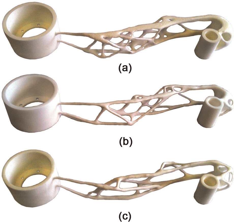
Although the optimization was performed using the properties of an aerospace grade aluminium alloy, the topologies were manufactured from a polyamide material (PA2200, EOS), with a Young’s modulus of 1700 ± 150 N/mm.^2,23 Topologies corresponding to those in Figure 9(a), (e) and (g) were manufactured, and the resultant parts are shown in Figure 23.

Figure 23.

Optimal topologies manufactured using selective laser sintering where $R\prime$ is (a) 1.5, (b) 2.5 and (c) 3.0.

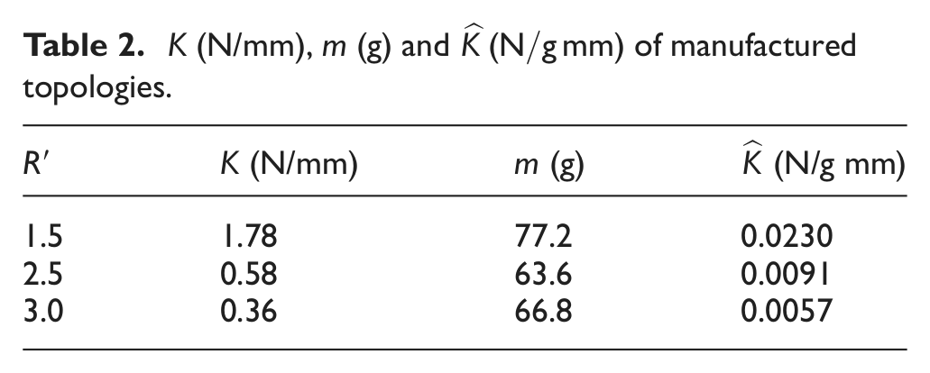
Using a polymer rather than a metal necessitated a lower load during testing, however, within the range tested, linear deformation was observed, enabling the results from the experimental testing to be compared with the FEA by scaling with the ratio of the modulus of the aluminium to that of the polymer. Comparison of the experimental deformation with that from a FE model of the corresponding smoothed topology yielded errors of less than 5%, thus confirming the accuracy of the analysis and manufacture. The most likely sources of the errors are variations in the density in the manufactured part and small differences in the assumed and experimental boundary conditions. A summary of the results from the experimental testing is presented in Table 2. It can be seen that the stiffness of the optimal structure, $K$ , increases with decreasing $R\prime$ . This is in agreement with the trend seen in the TO studies, for example, see Figure 11, where $C_{\infty }$ is inversely proportional to stiffness. As mentioned previously, modifications to the geometry to enable manufacture resulted in changes in the volume fraction, and hence mass, of the structure, as shown in Table 2. Therefore, a fairer comparison of the performance of the structures can be made using a specific stiffness, $\hat{K}$ , defined as the stiffness-to-mass ratio. From Table 2, it can be seen that $\hat{K}$ also increases with decreasing $R\prime$ , further validating the trends noted in the BESO parametric study.

Table 2.

K (N/mm), m (g) and $\hat{K}(\text{N}/\text{g mm})$ of manufactured topologies.

$R\prime$	$K$ (N/mm)	$m$ (g)	$\hat{K}$ (N/g mm)
1.5	1.78	77.2	0.0230
2.5	0.58	63.6	0.0091
3.0	0.36	66.8	0.0057

Structural integrity of topologically optimized design

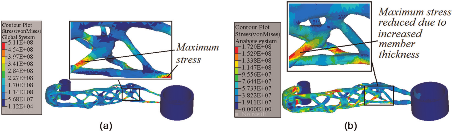
As mentioned in the ‘Introduction’ section, TO normally constitutes the first phase of a design optimization process. A second phase would commonly involve a shape and/or size optimization to ensure structural integrity and manufacturability of the final design. With AM, manufacturing constraints are less important than in most traditional manufacturing methods; however, it is useful to demonstrate how a structure from the TO in the present study could be modified to ensure structural integrity. Figure 24(a) shows the results of a FE stress analysis of the topology shown in Figure 23(a).

Figure 24.

von Mises stress distribution in TO structure (a) before and (b) after shape optimization to comply with stress constraint.

It can be seen that in two of the members, the von Mises stress is 511 MPa, which is close to the yield strength of a typical aerospace aluminium alloy, which in this case is taken to be 530 MPa. ²⁴ Assuming a safety factor of 2.5, a maximum von Mises stress constraint of 212 MPa can be imposed on the structure. Modification of the structure to satisfy this constraint can be achieved using an automated shape or size optimization algorithm; however, it is often quicker to achieve this manually when working with a parametric CAD model. A modified structure is shown in Figure 24(b) in which the members violating the stress constraint have been modified, with a resulting maximum stress of 172 MPa in the modified structure, which thus satisfies the structural integrity constraint. This step will increase the volume, and hence, weight of the structure. In this case, $V^{*}$ after the structural integrity modifications has increased from 0.11 to 0.17.

Conclusion

A comprehensive analysis of the topological optimization of an industrial aerospace part for AM has been performed. Contrary to the usual approach of removing fine structure, here it is both beneficial and realizable, suggesting the filter radius should be as small as possible, while avoiding checkerboarding to create a structure with fine features and high complexity. The evolution had little effect on the quality of the solution in this case, suggesting the selection of a high evolution rate, $v$ , to reduce computational time. The studies show the potential of TO for AM processes, with significant gains in design time and mechanical performance with a small marginal cost. Previously published studies using BESO algorithms for TO have tended to be restricted to basic problems with simple domains. This article shows that a BESO TO can be effectively used to optimize an industrial component, and that the dependence of the resultant optima on the optimization parameters can be used to drive the solution to a form suited to a particular manufacturing process.