Sage Journals: Discover world-class research

Abstract

Currently, a lack of interpretation tools and methodologies hinders the ability to assess the performance of a single piece of equipment or a total system. Therefore, a reliability, availability, and maintainability analysis must be combined with a quantitative reliability impact analysis to interpret the actual performance and identify bottlenecks and improvement opportunities. This article proposes a novel methodology that uses reliability, availability, and maintainability analysis to quantify the expected impact. The strengths of the failure expected impact methodology include its ability to systematically and quantitatively assess the expected impact in terms of reliability, availability, and maintainability indicators and the logical configuration of subsystems and individual equipment, which show the direct effects of each element on the total system. This proposed analysis complements plant modeling and analysis. Determining the operational effectiveness impact, as the final result of the computation process, enables the quantitative and unequivocal prioritization of the system elements by assessing the associated loss as a “production loss” regarding its unavailability and effect on the system process. The Chilean copper smelting process study provides useful results for developing a hierarchization that enables an analysis of improvement actions that are aligned with the best opportunities.

Keywords

Reliability analysis failure reliability engineering maintenance industrial engineering life cycle assessment

Introduction and background

Literature review

The effectiveness of production processes and their associated equipment is an important tool for assessing total system effectiveness,¹ which is generally measured according to the results of reliability and availability indicators and life cycle economic analysis.² The total equipment effectiveness indicator measures the productive efficiency using the control parameters as a basis for calculating the fundamentals of industrial production: availability, efficiency, and quality.³

In the current literature, several investigations have been performed to identify the principal factors that directly affect the maximization of economic benefits; these factors converge at the empirical consideration of reliability, availability, and maintainability (RAM) indicators. The traditional reliability analyses that are based on logical and probabilistic modeling contribute to the improved key performance indicators (KPIs) of a system,⁴ which directly influence optimal operation designs.⁵ However, many alternatives are available for system reliability analyses that employ analytical techniques, such as Markov models,⁶ Poisson models,⁷ universal generating function (UGF) and decision diagram.⁸ This systematic study is based on techniques such as reliability block diagrams (RBDs),^9,10 fault trees (FTs),¹¹ reliability graphics (RGs),¹² and Petri nets (PNs);¹³ these techniques can be used to determine logical relationships that underlie the behavior or dynamics of a process.

As an example, the productive processes in the mining industry have numerous equipment and systems, rendering a systematic analysis of the plant more difficult.⁴ Different analysis methodologies, such as the RBD methodology,^9,10 have been developed and extensively applied in the mining sector due to their adaptability in representing complex arrangements and environments with large amounts of equipment, simplifying reliability analysis. For the correct development of an RAM analysis, a complete scan of the data must be performed to fit the data to a statistical model and to then obtain key indicators.¹⁴ Using a maintenance management support tool, different improvement opportunities can be identified, and recommendations can be offered to develop the most appropriate actions.¹⁵

The Birnbaum importance measure (IM)¹⁶ ranks the components of the system with respect to the impact of their failure on the overall system’s performance; however, its application is primarily related to epistemic uncertainties.

Interpretation tools and methodologies for understanding the performance of a single piece of equipment and a total system are lacking; this deficiency is even more pronounced when the selected analysis process has been disaggregated on many levels, and each level has been disaggregated across several pieces of equipment. Therefore, an RAM analysis must be combined with a quantitative reliability impact analysis to determine the real performance and identify bottlenecks and opportunities for improvement.

Motivation of work

This article proposes an integral and quantitative innovative methodology to analyze the RAM and plant failure expected impact (FEI). The FEI analysis is related specifically to production capacity and the effect of preventive and corrective maintenance intervention on system availability. This proposal designs a novel algorithm to compute an impact index based on the frequency of failures associated, with the reliability and maintainability of the machinery and the expected impact according to different scenarios and configurations. This impact index, based on a probabilistic approach, defines the expected condition of the item in the system from a perspective of evaluation of its possible states (intrinsic behavior) and related to the logical and functional configuration of the system. This approach enables an overall comparison of elements and the prioritization of those elements, as well as a partial effectiveness assessment.

What is the motivation for applying the FEI methodology?

In the finance area, for example, when a single stock of the NASDAQ index has a variation price of 10% and this stock represents 5% of the index composition, the NASDAQ index increases by only 0.5%. Developing a similar analysis over an “element” failure and determining the system consequences are simple when the “elements” have a serial configuration. If the configuration employs redundancy logic, the result is uncertain and dependent on the reliability and maintainability of the elements that compose the subsystem. The FEI methodology solves this problem by proposing four steps and applying them to a mining process—specifically, a copper smelting process (CSP) in Chile. Related to failure impact methodology, a novel algorithm is proposed to compute a failure impact index for the total availability performance of the system based on the reliability (frequency of failures), maintainability (downtime), and availability of the elements. This impact index defines the expected condition of the item in the system by evaluating its possible states (intrinsic behavior) and the logical and functional configuration of the system. This analysis enables a total comparison of the elements, their prioritization, and a failure impact evaluation.

Scope of work

The two key indicators of FEI methodology are outlined in Figure 1, which incorporates general formulas for analysis and calculation. This methodology seeks to explain the level of responsibility for a failure in a single piece of equipment (b3) for system inoperability from a historical perspective. Two important steps are included:

Explain the effect of a single failure (downtime Ti of equipment b3) in terms of the single downtime propagation in the system (equivalent downtime ti). This indicator is named the expected downtime factor propagation (E-DFP).

Explain the effect of a single downtime propagation (equipment b3) on the total downtime of the system (downtime responsibility). This indicator is named the expected operational criticality index (E-OCI).

Figure 1.

Expected impact scheme.

A copper smelting plant in Chile is examined as a case study. The smelting process is one of the most important and critical phases in any mineral processing system, especially in copper plants.¹ The selected mining process is divided into four main subsystems: drying, concentrate fusion, conversion, and refining.

This article is structured as follows: section “FEI methodology” describes the reliability assessment based on the FEI methodology and presents its conceptual and mathematical basis, section “Case study” introduces and develops the case study according to the methodology, and section “Conclusion” explains the main results and conclusions.

FEI methodology

The FEI methodology should consider the joint processes that are necessary for identifying improvement opportunities and generating maintenance recommendations. These processes can be summarized in four steps: data cleaning, data management, RAM analysis, and FEI quantification (E-OCI and E-DFP) and decision making.

Data cleaning

The first step is to purge and filter the obtained data to improve the data quality (missing values, usefulness records, and erroneous data).¹⁷

Data management

To achieve an efficient data management, some methodologies can be considered based on the equipment (historical reparable behavior). A repairable system after a failure scenario can be restored to its functioning condition (perfect and imperfect) by maintenance actions, with the exception of the replacement¹⁸ (nonreparable item). A reparable system is defined as follows: “A system that, after failing to perform one or more of its functions satisfactorily, it can be restored to fully satisfactory performance by any method other than replacement of the entire system.”¹⁹ The model and analysis of reparable equipment have high importance, mainly in order to increase the performance oriented to reliability and maintenance as part of the cost reduction in this last item. Depending on the type of maintenance given to equipment, it is possible to find five cases:²⁰

Perfect maintenance or reparation. Maintenance operation that restores the equipment to the condition “as good as new.”

Minimum maintenance or reparation. Maintenance operation that restores the equipment to the condition “as bad as old.”

Imperfect maintenance or reparation. Maintenance operation that restores the equipment to the condition “worse than new but better than old.”

Over-perfect maintenance or reparation. Maintenance operation that restores the equipment to the condition “better than new.”

Destructive maintenance or reparation. Maintenance operation that restores the equipment to the condition “worse than old.”

For a perfect maintenance, the most common developed model corresponds to the perfect renewal process (PRP). In this, we assume that repairing action restores the equipment to a condition as good as new and assumes that times between failures in the equipment are distributed by an identical and independent way. The most used and common model PRP is the homogeneous Poisson process (HPP), which considers that the system neither ages nor spoils independently of the previous pattern of failures. That is to say, it is a process without memory. Regarding case b, “as bad as old” is the opposite case to what happens in case a, “as good as new,” since it is assumed that the equipment will stay after the maintenance intervention in the same state than before each failure. This consideration is based on that the equipment is complex, composed by hundreds of components, with many failure modes and the fact that replacing or repairing a determined component will not affect significantly the global state and age of the equipment. In other words, the system is subject to minimum repairs, which does not cause any change or considerable improvement. The most common model to represent this case is through nonhomogeneous Poisson process (NHPP), in this case the most used model to represent NHPP is called “Power Law.” In this model, a Weibull distribution is assumed for the first failure and that later, it is modified over time. Although the models HPP and NHPP are the most used, they have a practical restriction regarding its application since a more realistic condition after a repairing action is what we find between both: “worse than new but better than old.” In order to find a generalization to this situation and not distinguishing between HPP and NHPP, it was necessary to create the generalized renewal process (GRP).²¹ The main objective of this stage is to generate parameters evaluation and basic indicators.

RAM analysis

Reliability analysis

Different alternatives have been proposed for the individual and systemic logical–functional representations of processes.⁴ Modeling a complex system using RBDs is a well-known method that has been adopted for different applications in system reliability analysis.^5,22 An RBD is constructed after performing a logical decomposition of a system into subsystems; the RBD is constructed to express reliability logics such as series, redundancy, and standby in a network of subsystems. RBDs are considered to be a modeling tool that is consolidated and available for the normal duties of reliability analysis. The RBD analysis methodology^9,10 is used extensively in the mining sector due to its adaptability for representing complex provisions and environments with large amounts of equipment. An RBD can be applied in addition to other reliability techniques, such as a fault tree analysis (FTA).

Maintainability analysis

Maintainability performance is defined as

the ability of an item under given conditions of use to be retained in, or restored to, a state in which it can perform a required function, when maintenance is performed under given conditions and using stated procedures and resources.²³

The “given conditions” refer to the conditions in which the item is used and maintained, for example, climate conditions, support conditions, human factors, and geographical location. The maintainability of equipment can be represented and understood as a probability distribution of the maintenance completion time. Parametric methods have been used to analyze historical time to repair (TTR) datasets in many case studies.²⁴

Availability analysis

According to Dhillon,⁵ availability is the probability that the equipment is available as required. Assuming that the required equipment must always be operating and that maintenance orders are immediately executed after a failure, the expected availability of the determined equipment can be defined²⁵

\begin{array}{l} A (t) = \frac{S y s t e m u p t i m e}{S y s t e m u p t i m e + S y s t e m d o w n t i m e} \\ \approx \frac{M T T F}{M T T F + M T T R} \end{array}

(1)

Availability is probably the most important parameter because it is directly related to the equipment performance, especially in a production environment that is based on volume, such as the mining industry. In this environment, the rate of production, among other variables, determines the level of benefit that is derived from the exercises. Monte Carlo simulation is used as a modeling framework to represent the realistic features of the equipment and the complex behavior of high-dimensional systems to obtain the performance indicators for the availability.⁴

FEI quantification and decision making

To implement an efficient asset management, an item classification should be developed based on criteria such as direct and indirect costs, failure rate, and operational impact. The objective is to identify the relevant elements in making priority maintenance decisions and efficiently allocating resources. Many techniques exist for asset hierarchy, and each technique has advantages and disadvantages that depend on the operation context.⁴ For this proposal, the authors present a novel quantitative methodology for measurement based on reliability impact using previous results of RAM analysis.

FEI methodology

In this phase, the first indicator is the E-OCI of each element in the system, which is determined by decomposing the global index and each subsystem index²⁶ on the following levels

E - O C I_{s y s t e m i = 0} = 1

(2)

Equation (2) represents the start of the process considering the E-OCI as a 100%. Then, the breakdown of each level begins with the following equations

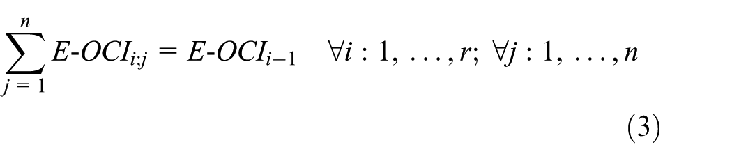
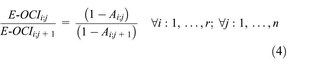
\sum_{j = 1}^{n} E - O C I_{i; j} = E - O C I_{i - 1} \forall i : 1, \dots, r; \forall j : 1, \dots, n

(3)

In equation (3), the E-OCI of a level is distributed in all the elements that composed it, all this to keep the consistence of the impact quantification. To determine the E-OCI of each element of the lower level, it is necessary to develop equation (4), which considers the distribution by an unavailability factor. In this sense, the most unavailable element of the lower level obtains a bigger proportion of the E-OCI from the upper level

\frac{E - OC I_{i; j}}{E - OC I_{i; j + 1}} = \frac{(1 - A_{i; j})}{(1 - A_{i; j + 1})} \forall i : 1, \dots, r; \forall j : 1, \dots, n

(4)

where E-OCI_i;j is the E-OCI for element j (from 1 to n) that is included in decomposition level i (from 1 to r) and $A_{i; j}$ is the expected availability for element j (from 1 to n) that is included in decomposition level i (from 1 to r).

In simple terms, the E-OCI shows the final contribution of each element toward mitigating the system’s lack of effectiveness based on the production capacity loss. When considering a lower detail level, such as level r, the sum of all E-OCI values is 100% of the system

\sum_{i = 1}^{r} \sum_{j = 1}^{n} E - OC I_{i; j} = 1

(5)

Once the E-OCI_i;j of each item is known, its level of impact is divided into two main aspects: frequency (by the unavailability of the element) and consequence (by the impact of the element). The consequence is E-DFP_i;j, which represents the effect on system j of element i stopping. The effect of stopping element i may have different results on system j depending on the state of the elements that are also on level i. Particularly, equation (7) is deducted from the definition of E-OCI and the relation between the element and system unavailability (equation (6))

E - OC I_{i; j} = \frac{(1 - A_{i; j}) * E - DF P_{i; j}}{(1 - A_{system})}

(6)

E - DF P_{i; j} = \frac{E - OC I_{i; j} * (1 - A_{system})}{(1 - A_{i; j})}

(7)

Figure 2 shows the FEI methodology and each phase of the process. Table 1 shows a comparative analysis between the main criticality and the operative impact methodologies.

Figure 2.

FEI methodology.

Table 1.

Comparison of operative impact assessment methodologies.

Methodology	Typology	Focus	Failure effect estimation	Flexibility
Failure tree¹¹	Qualitative	Individual	Failure analysis	High
US Department of Defense²⁷	Qualitative	Individual	Failure analysis	High
Crespo et al.²⁸ proposal	Quantitative	Systemic	Expert criteria (1–5)	Medium
FEI²⁶	Quantitative	Systemic	Probabilistic impact analysis	High

FEI: failure expected impact.

Case study

For the analytical development of this case study, the selected process and equipment in the analysis are presented to develop the logical–functional sequence RBD due to the complexity of the system with a large amount of equipment. Then, the time to failure (TTF) and the TTR are analyzed to validate and identify trends and correlations. The parameterization is performed according to the most suitable stochastic model, which represents both the nature of the failure and the process of repairing the equipment. The FEI is individually and systematically developed to obtain the main indicators and identify the equipment with the highest impacts on the process.

The data were collected over a period of 16 months using the Plant Maintenance Module of SAP Enterprise Resource Planning software (SAP-PM) report from the mining industry in Chile. Considering that current automatic capture systems provide rich and complete data with respect to operational parameters, focused on prognosis and health management application, data related to the state of the asset, specific process parameters, and downtimes. This data repository is linked with information related to work notifications and work orders. Accordingly, an enterprise resource planning (ERP) solution permits the complete integration of information flow from all functional areas by means of a single database that is accessible through a unified interface and channel communication. Hence, it is possible to apply the proposed methodology using this consolidated database validating the quality and quantity of the information.

The CSP case study

The case study is the smelting process of a mine in Chile; the first stage of this process is smelting ore, which contains a concentration of approximately 26% copper. The pyro-metallurgical operations, which enable the extraction of metallic copper, are performed in type A converters (the melting process), type B converters (the conversion process), slag cleaning furnaces (the copper recovery process), fire refinement stoves (the refined copper preparation process), and anodic furnaces (the anodic copper preparation process). The nominal production capacity of the smelting process is 60 tons/h. The resulting gases from the fusion conversion process are treated in gas cleaning plants, which also produce sulfuric acid that is primarily marketed in the mining industry in the northern region of Chile. Therefore, the portfolio of products obtained through these processes includes copper plates with 99.7% purity, fire refined copper ingots with 99.9% purity and sulfuric acid derived from the processing of smelter gases (Table 2). The analytical development of the case study uses the main operational flow of the concentrate in the smelting process, which is represented by the equipment and subprocesses shown in Figure 3. The mining subprocesses that are considered in this article are drying, concentrate fusion, conversion, and refining.

Table 2.

CSP information.

Equipment	Label	Basic function	Capacity (ton/h)
Equipment	Label	Basic function	Nominal	Maximum
Dryer 1	D1	Drying	30	60
Dryer 2	D2	Drying	30	60
Type A converter 1	CA1	Conversion type A	30	60
Type A converter 2	CA2	Conversion type A	30	60
Type B converter 1	CB1	Conversion type B	20	30
Type B converter 2	CB2		20	30
Type B converter 3	CB3		20	30
Refining anode furnace 1	RAF1	Refining A	30	60
Refining anode furnace 2	RAF2	Refining A	30	60
Anode furnace 1	AF1	Refining B	30	60
Anode furnace 2	AF2	Refining B	30	60

CSP: copper smelting process.

Figure 3.

Case study process diagram.

Modeling the system

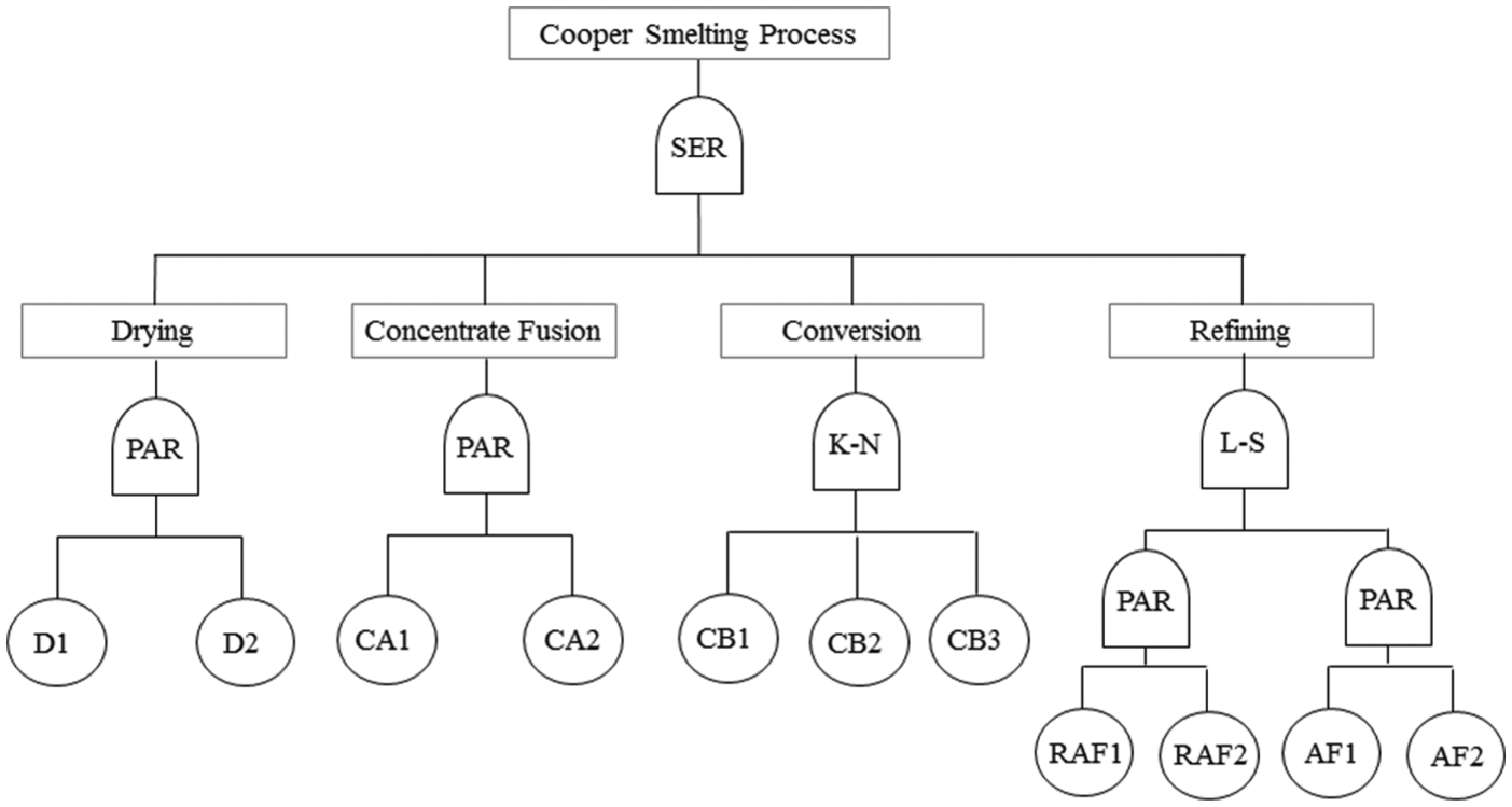
The logic behind the process operations can be represented using FT diagrams, which enable the subsequent development of the RBD configuration. According to Table 1, the FT is constructed as shown in Figure 4:

Figure 4.

FT representation of the process.

According to Figure 2, the smelting process is composed of four subsystems arranged serially: the drying subsystem (DS), which consists of two dryers in full redundancy; the concentrate fusion subsystem (CFS), which consists of two type A converters in full redundancy; the conversion subsystem (CS), which consists of three type B converters in a 3-2 configuration with partial redundancy; and the refining subsystem (RS), which consists of two work lines that separate the refining anode furnace (RAF) production from the anode furnace (AF) plate production, with a load distribution of 60% and 40%, respectively. Each subprocess is composed of two elements in total redundancy. The classification for the reliability analysis of the CSP is presented in the FT diagram.

The quantitative analysis of the CSP considers the operating conditions, failure data, maintenance times, and other functional information needed to estimate the RAM indicators for each piece of equipment, each subsystem, and the total system. Reliability analysis was performed using traditional algorithms.²⁶

Data analysis

The collected data include TTF and TTR for each equipment. The next step in data management is to determine the nature of the equipment that is involved in the process. In this case, all of the equipment uses the dynamics of serviceable equipment, and its subsequent distribution must be selected using relevant stochastic models²⁹ according to the behaviors of the data in terms of trend and independence.

Trend and correlation analysis

Analyzing the data of the equipment that is involved in the process, the independence and trend indicators are calculated. The calculated values of the test statistics for all of the equipment failures and repair data are listed in Table 3. Using the null hypothesis of an HPP, in which the test statistic U is χ² distributed with 2(n − 1) degrees of freedom, the null hypothesis is not rejected at a 5% level of significance in most of the equipment. The statistical results show that the datasets for the majority of the equipment, with the exceptions of the TTF data for CB3, RAF1, and AF1, show no trends or serial correlation. Therefore, the independent and identically distributed (i.i.d.) assumption is rejected for these equipment. Identical results were obtained from the graphical trend analysis.¹⁴

Table 3.

Statistical results for TTF and TTR data.

Subsystem	Equipment	Dataset	Degrees of freedom	Statistic U	Rejection of null hypothesis at a 5% level of significance
DS	D1	TTF	96	97.25	Not rejected (>76.11)
	D1	TTR	96	82.21	Not rejected (>74.40)
	D2	TTF	66	57.32	Not rejected (>52.34)
	D2	TTR	66	51.31	Not rejected (>47.85)
CFS	CA1	TTF	62	47.56	Not rejected (>39.65)
	CA1	TTR	62	45.44	Not rejected (>40.67)
	CA2	TTF	56	46.17	Not rejected (>38.95)
	CA2	TTR	54	45.76	Not rejected (>38.65)
CS	CB1	TTF	62	49.13	Not rejected (>33.56)
	CB1	TTR	62	50.17	Not rejected (>34.55)
	CB2	TTF	70	54.23	Not rejected (>47.36)
	CB2	TTR	70	49.95	Not rejected (>42.72)
	CB3	TTF	92	89.34	Rejected (<92.71)
	CB3	TTR	90	87.36	Not rejected (>70.23)
RS	RAF1	TTF	70	52.14	Rejected (<53.11)
	RAF1	TTR	70	56.22	Not rejected (>52.34)
	RAF2	TTF	68	49.76	Not rejected (>42.57)
	RAF2	TTR	68	47.66	Not rejected (>43.54)
	AF1	TTF	62	58.27	Rejected (<59.56)
	AF1	TTR	62	60.22	Not rejected (>53.33)
	AF2	TTF	54	41.56	Not rejected (>39.44)
	AF2	TTR	52	41.75	Not rejected (>37.72)

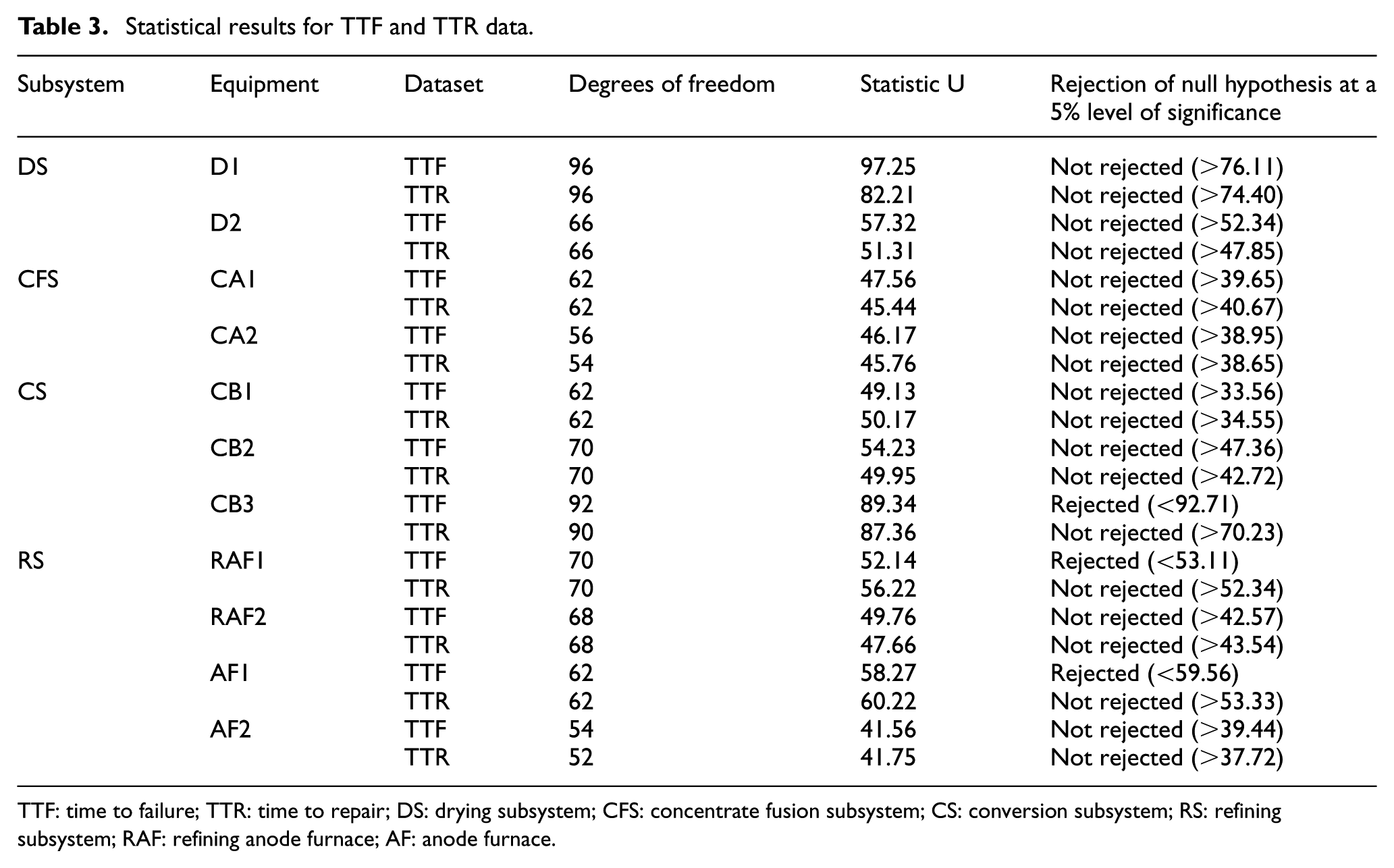
TTF: time to failure; TTR: time to repair; DS: drying subsystem; CFS: concentrate fusion subsystem; CS: conversion subsystem; RS: refining subsystem; RAF: refining anode furnace; AF: anode furnace.

Distribution fitting and calculation of basic indicators

The definition of the probability distributions is commonly used to describe the equipment failure and repair processes. Different types of statistical distributions were examined, and their parameters were estimated using MATLAB.³⁰ A statistical goodness-of-fit test was performed to define the distributions of the operating times and TTR. In particular, Kolmogorov–Smirnov tests²⁵ at a significance level of a = 0.1 were required to be satisfied for p = 0.1 at each setting. The null hypothesis H0 is as follows: the data follow a normal, log-normal, exponential, or Weibull distribution.

The equipment trend data should be analyzed using a stochastic model for reparable elements. The NHPP model used in this study is based on the power law process (PLP). The χ² test and the Kolmogorov–Smirnov test were classically encountered to validate the best-fit distribution.³¹ The parameters that were estimated from the failure data are listed in Table 4.

Table 4.

Fitting distributions of the TTF and TTR data.

Equipment	Best fit (TTF data)
Equipment	Distribution	p value (K-S)	Parameter 1	Parameter 2	MTTFi
D1	Weibull	0.29	α = 238	β = 1.13	228
D2	Weibull	0.17	α = 224	β = 1.2	211
CA1	Exponential	0.14	α = 253	β = 1.6	227
CA2	Weibull	0.43	α = 330	β = 1.4	300
CB1	Exponential	0.32	α = 256	β = 1	256
CB2	Weibull	0.29	α = 792	β = 1.34	722
CB3	NHPP-PLP	0.31	α = 402	β = 1.32	269
RAF1	NHPP-PLP	0.28	α = 351	β = 1.27	211
RAF2	Weibull	0.40	α = 144	β = 1.30	133
AF1	NHPP-PLP	0.23	α = 324	β = 1.31	203
AF2	Exponential	0.61	α = 315	β = 1	315
Equipment	Best fit (TTR data)
	Distribution	p value (K-S)	Parameter 1	Parameter 2	MTTRi
D1	Lognormal	0.57	µ = 0.478	σ = 2.24	4.94
D2	Lognormal	0.24	µ = 0.731	σ = 1.3	3.97
CA1	Lognormal	0.71	µ = 0.940	σ = 1.8	6.29
CA2	Normal	0.61	µ = 4.8	σ = 1.2	4.84
CB1	Lognormal	0.66	µ = 1.31	σ = 1.57	8.12
CB2	Lognormal	0.35	µ = 1.45	σ = 2.02	11.71
CB3	Normal	0.69	µ = 7.33	σ = 1.4	7.33
RAF1	Lognormal	0.21	µ = 1.44	σ = 1.1	7.31
RAF2	Lognormal	0.61	µ = 0.872	σ = 1.24	4.41
AF1	Lognormal	0.45	µ = 1.31	σ = 1.45	7.65
AF2	Lognormal	0.24	µ = 0.91	σ = 1.7	5.82

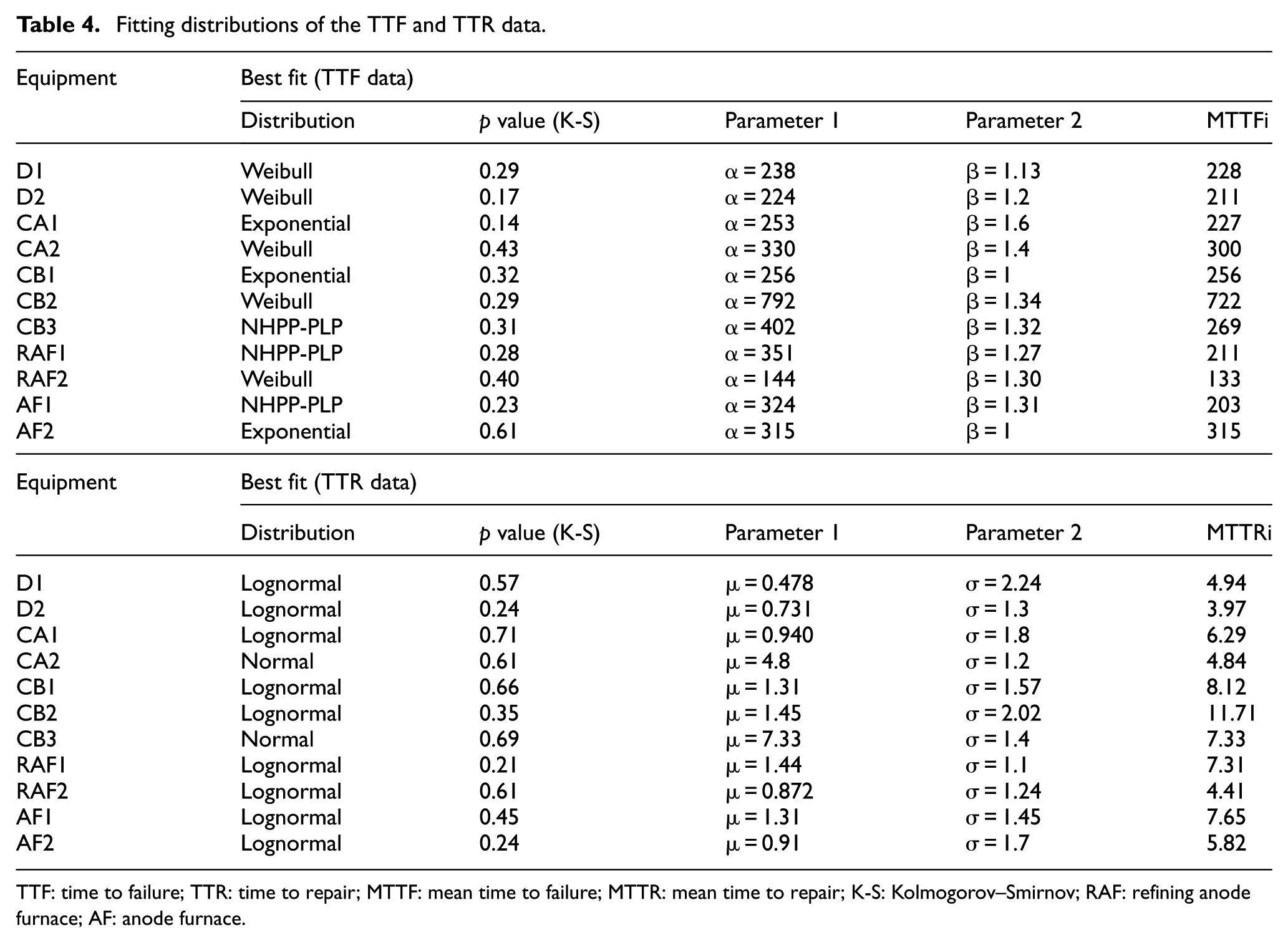
TTF: time to failure; TTR: time to repair; MTTF: mean time to failure; MTTR: mean time to repair; K-S: Kolmogorov–Smirnov; RAF: refining anode furnace; AF: anode furnace.

Table 4 also lists the basic indicator of reliability, which is the mean time to failure (MTTF), the basic indicator of maintainability, which is the mean time to repair (MTTR), and the respective parameters of the fitted curves.

According to the traditional setting (no trend), the reliability parameters of the fitted curves (α, β), which are based on the life cycle theory,³¹ show that the equipment are in different phases of the bathtub curve. β = 1 is related to a constant failure rate or “useful” life phase; β > 1 is the phase in which the failure rate typically increases, and additional service and maintenance are needed. In the “wear-out” life phase, a technical and economic assessment is required to determine the need for possible replacement, and in the β < 1 phase, the component failure rate decreases over time. Early life cycle problems are often due to failures in design, incorrect installation, and operation by poorly trained operators. Therefore, the statistical information obtained from the curve fitting should be used to estimate the system performance instead of explaining individual equipment behavior.

The probability distribution that is commonly used to represent repair times is the normal-logarithmic distribution, which explains the variability of repair by two phenomena:³² the variation of the time associated with accidental factors (negative exponential distribution) and the factors related to typical repair (normal distribution).

System reliability analysis

CSP is divided into four subsystems, which comprise a logical–functional configuration series, that is, all subsystems must be operating to ensure that the process performs properly. Subsystem and system reliability is generally calculated using the standard RBD formulas.^5,22

Table 5 presents the main reliability results for different operating times. The reliability results for the main subsystem and total system are shown graphically in Figure 5.

Table 5.

Reliability evaluation of the CSP.

	R(0)	R(50)	R(100)	R(150)	R(200)	R(250)	R(300)	R(350)	R(400)
System	1.000	0.948	0.785	0.568	0.360	0.196	0.088	0.031	0.009
DS	1.000	0.976	0.901	0.794	0.674	0.556	0.449	0.356	0.278
D1	1.000	0.842	0.687	0.552	0.440	0.347	0.273	0.213	0.166
D2	1.000	0.848	0.684	0.539	0.418	0.320	0.242	0.181	0.135
CFS	1.000	1.000	0.999	0.987	0.943	0.833	0.643	0.412	0.218
CA1	1.000	0.928	0.797	0.648	0.503	0.375	0.269	0.186	0.125
CA2	1.000	1.000	0.993	0.964	0.885	0.732	0.512	0.278	0.106
CS	1.000	0.987	0.942	0.869	0.778	0.679	0.580	0.486	0.401
CB1	1.000	0.823	0.677	0.557	0.458	0.377	0.310	0.255	0.210
CB2	1.000	0.979	0.946	0.907	0.864	0.820	0.773	0.727	0.681
CB3	1.000	0.953	0.882	0.802	0.721	0.640	0.564	0.492	0.426
RS	1.000	0.984	0.925	0.834	0.728	0.622	0.523	0.436	0.360
RAF subsystem	1.000	0.981	0.911	0.801	0.677	0.556	0.449	0.359	0.284
RAF1	1.000	0.917	0.807	0.694	0.588	0.491	0.405	0.331	0.268
RAF2	1.000	0.777	0.537	0.348	0.216	0.129	0.075	0.042	0.023
AF subsystem	1.000	0.988	0.948	0.884	0.806	0.721	0.635	0.551	0.473
AF1	1.000	0.917	0.807	0.694	0.588	0.491	0.405	0.331	0.268
AF2	1.000	0.853	0.728	0.621	0.530	0.452	0.386	0.329	0.281

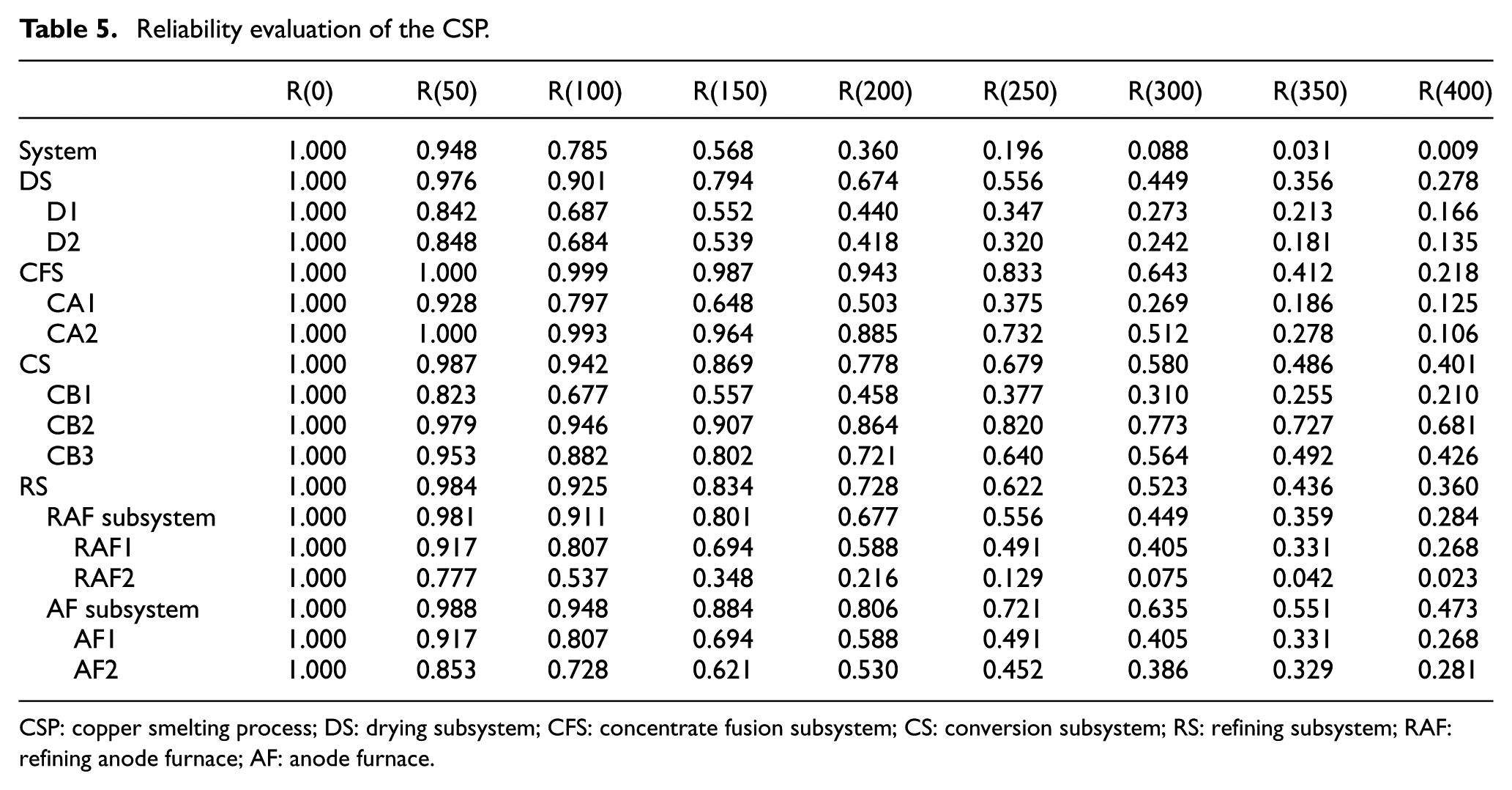
CSP: copper smelting process; DS: drying subsystem; CFS: concentrate fusion subsystem; CS: conversion subsystem; RS: refining subsystem; RAF: refining anode furnace; AF: anode furnace.

Figure 5.

Reliability curves for the main subsystems in the CSP.

Through numerically and graphically analyzing the reliability results, the DS and RS subsystems show an accelerated decrease in reliability compared with the other subsystems (exponential behavior). The CS subsystem presents the best condition due to the redundant configuration of the subsystem and the distinctly reliable behavior of the equipment. During the first 300 h, the CFS subsystem presents the most reliable behavior due to its redundancy; after this time, the reliability decreases exponentially (wear-out behavior).

To identify opportunities to improve the reliability, processes should focus on subsystems with less reliability over time, that is, DS and RS. This information is the key for defining the intervals for preventive interventions. For example, if the reliability defined by an organization to develop the preventive intervention of critical equipment ranges between 75% and 80%, the planning activities for the DS subsystem should range between 75 and 100 h of operation. However, the examined system presents an important level of redundancy in three of its subsystems, which should also be considered when evaluating and defining future maintenance policies. In practical terms, a corrective policy is generally assumed in redundant systems. However, to reach this conclusion, individual assessment and identification of critical subsystems and equipment as well as the real costs of preventive and corrective interventions are required.⁵

System maintainability analysis

In terms of individual analyses, the maintainability has an important effect on the equipment and systemic availability results.²³ For each element, TTR and MTTR_i are required for the next analysis. Table 5 lists the parametric information for computing the MTTR_i.

System availability analysis

With the information obtained from the curve adjustments, the expected availability^5,22,33 was analyzed. Table 6 presents the results of the expected availability calculations for the equipment, subsystems, and system.

Table 6.

Expected availability calculation.

	MTTF (h)	MTTR (h)	Availability (%)	Subsystem availability (%)	System availability (%)
System					95.17
DS				98.66
D1	227.69	4.94	97.88
D2	210.71	3.98	98.15
CFS				98.62
CA1	226.83	6.30	97.30
CA2	299.95	4.80	98.42
CS				99.83
CB1	256.00	8.13	96.92
CB2	721.85	11.70	98.40
CB3	269.38	7.33	97.35
RS				97.99
RAF subsystem				97.77
RAF1	211.13	7.32	96.65
RAF2	133.00	4.45	96.77
AF subsystem				98.31
AF1	202.94	7.58	96.40
AF2	315.00	5.81	98.19

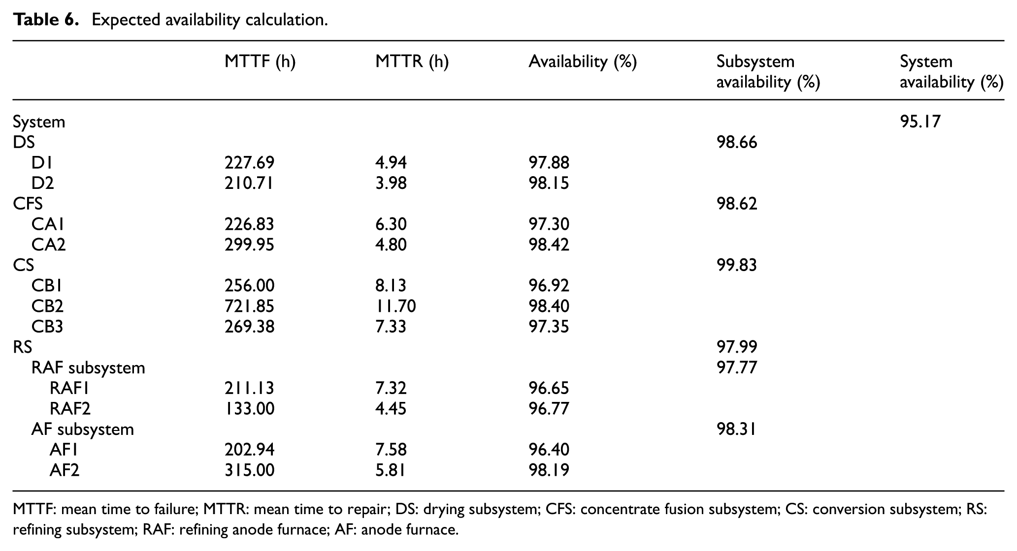
MTTF: mean time to failure; MTTR: mean time to repair; DS: drying subsystem; CFS: concentrate fusion subsystem; CS: conversion subsystem; RS: refining subsystem; RAF: refining anode furnace; AF: anode furnace.

According to the results, the subsystem with the least expected availability is RS, while CS has more availability. For this particular case, the availability results are consistent with the reliability results. Therefore, a practical mechanism is needed for identifying the highest E-OCI and integrating the RAM results.

According to the procedure in section “FEI methodology” and equations (2)–(6), the impacts of each piece of equipment, each subsystem, and the system are presented in Table 7.

Table 7.

Calculation of E-OCI and E-DFP.

	E-OCI (%)	E-DFP (%)
System	100.00	100.00
DS	27.27	98.35
D1	14.57	33.09
D2	12.71	33.09
CFS	28.22	98.35
CA1	17.82	31.85
CA2	10.39	31.85
CS	3.47	98.35
CB1	1.46	2.29
CB2	0.76	2.29
CB3	1.26	2.29
RS	41.04	98.35
RAF subsystem	24.62	53.36
RAF1	12.53	18.05
RAF2	12.10	18.05
AF subsystem	16.42	46.78
AF1	10.92	14.65
AF2	5.50	14.65

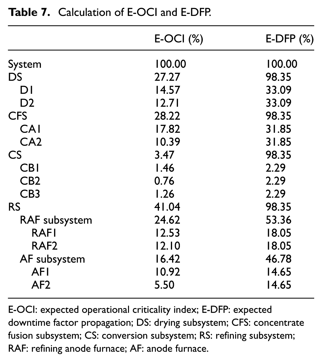
E-OCI: expected operational criticality index; E-DFP: expected downtime factor propagation; DS: drying subsystem; CFS: concentrate fusion subsystem; CS: conversion subsystem; RS: refining subsystem; RAF: refining anode furnace; AF: anode furnace.

Table 7 shows that D1 explains 14.57% of the lack of effectiveness of the system, which is expressed as the E-OCI; each D1 failure results in an expected 33.09% loss of production capacity for the total system, which is expressed as the E-DFP. Both impact indices are dependent on the behavior of the equipment in terms of the RAM results, operational context, and logical dependencies as well as the indicators for the other pieces of equipment in their subsystem (immediately higher level). The E-DFP values for each subsystem are equal, which is attributed to the serial configuration of the system.

Using this analysis, the equipment and subsystems that generate the highest impact on the availability or production of the main system can be grouped together. However, the results are not distinct. Therefore, continuity with a dispersion analysis is proposed in which the X-axis corresponds to the unavailability and the Y-axis corresponds to the E-DFP. In this manner, the generated curves correspond to the expected operational criticality iso-impact curves.

First, an analysis is performed at the subsystem level (Figure 6); DS, CFS, CS, and RS have the same level of E-DFP because they are in series. Therefore, the unavailability of each subsystem creates a different E-OCI. The subsystems RAF and AF have a smaller E-DFP because they employ a load-sharing configuration (60% of the load and 40% of the load, respectively) in the RS subsystem.

Figure 6.

FEI methodology dispersion analysis for the subsystems.

Figure 7 shows the relatively low E-DFP for the equipment, which is attributed to the redundancy in each of the subsystems. Due to the serial configuration of all subsystems, the E-DFP values are all identical, with the exception of the RAF and AF subsystems, which have different capacities and operational contexts. The order of the subsystems in terms of operational effectiveness is RS, CFS, DS, and CS. At the individual level, the order of the equipment is as follows: CA1, D1, D2, RAF1, RAF2, AF1, CA2, AF2, CB1, CB3, and CB2.

Figure 7.

FEI methodology dispersion analysis for the equipment.

Conclusion

The reliability impact study is a relevant analysis to develop a decision-making process. Considering the standard methodologies, it is possible to establish that there are no formal criteria to identify the impact of each asset and its behavior or failure. So, it is necessary to define a KPI oriented to establish a hierarchy and determine the effectiveness of the KPI’s impact on the elements.

A deep reliability analysis requires quality and quantity of data; therefore, this article shows the importance of the quality of information that is available for analysis; the existing data should be audited to validate the previous analysis.

The FEI methodology has significant potential applications in several engineering problems, industrial realities, and productive sectors. FEI is a powerful tool for analysis and decision making for the various phases of an industrial project via life cycle cost (LCC) for design-oriented operations, such as capital expenditures (CAPEX) and operational expenditures (OPEX), which are associated with the improvement process.

The strengths of the FEI methodology include its ability to systematically and quantitatively assess the operational criticality in terms of the RAM indicators and the logical configuration of subsystems and individual equipment, which directly affect each element in the total system. This proposal complements plant modeling and analysis, from traditional methodologies. The E-OCI is the final result of the computation process, which enables the quantitative and unequivocal prioritization of the system elements to assess the associated loss as “production loss” regarding its unavailability and effect in the process. The latter concept enables estimating the E-DFP of the equipment to determine the individual effects of the detention and assess complex and redundant scenarios.

The case study provides useful results for developing a hierarchization that enables an analysis of improvement actions that are aligned with the best opportunities.

Considering the FEI methodology structure, it is possible to conclude that it is replicable in different application fields and can be easily automated. Rankings that are based on the expected impact in the operation are effective, recognize weaknesses and opportunities, and serve as the basis for action plans based on reliability and maintainability.

Footnotes

Appendix 1

Academic Editor: Shun-Peng Zhu

Declaration of conflicting interests

The author(s) declared no potential conflicts of interest with respect to the research, authorship, and/or publication of this article.

Funding

The author(s) received no financial support for the research, authorship, and/or publication of this article.

References

Asaki

Kinetic studies of copper flash smelting furnace and improvements of its operation in the smelters in Japan. Miner Process Extr M 1992; 11: 163–185.

Parra

Desarrollo de modelos de cuantificación económica del factor Fiabilidad en el coste total de ciclo de vida de un sistema de producción. Tesis Doctoral, Universidad de Sevilla, Sevilla, 2009.

Pham

(ed.). Handbook of reliability engineering. Piscataway: NJ: Springer, 2003.

Viveros

Zio

Arata

. Integrated system reliability and productive capacity analysis of a production line. A case study for a Chilean mining process. Proc IMechE, Part O: J Risk and Reliability 2012; 226: 305–317.

Dhillon

BS.

Maintainability, maintenance, and reliability for engineers. Boca Raton, FL: Taylor & Francis Group, 2006.

Welte

TM.

A rule-based approach for establishing states in a Markov process applied to maintenance modeling. Proc IMechE, Part O: J Risk and Reliability 2009; 223: 1–12.

Heinrich

Goodness-of-fit tests for the second moment function of a stationary multidimensional Poisson process. Statistics 1991; 22: 245–278.

Peng

Zhai

Xing

. Reliability of demand-based phased-mission systems subject to fault level coverage. Reliab Eng Syst Safe 2014; 121: 18–25.

Rausand

Hoyland

System reliability theory: models, statistical methods, and applications. 3rd ed.New York: Wiley, 2003.

10.

Guo

Yang

A simple reliability block diagram method for safety integrity verification. Reliab Eng Syst Safe 2007; 92: 1267–1273.

11.

Rauzy

Gauthier

Leduc

Assessment of large automatically generated fault trees by means of binary decision diagrams. Proc IMechE, Part O: J Risk and Reliability 2007; 221: 95–105.

12.

Distefano

Puliafito

Reliability and availability analysis of dependent-dynamic systems with DRBDs. Reliab Eng Syst Safe 2009; 94: 1381–1393.

13.

Volovoi

Modeling of system reliability Petri nets with aging tokens. Reliab Eng Syst Safe 2004; 84: 149–161.

14.

Jiang

Xie

Wei

. A modified method for risk evaluation in failure modes and effects analysis of aircraft turbine rotor blades. Adv Mech Eng. Epub ahead of print 22 April 2016. DOI: 10.1177/1687814016644579.

15.

Barberá

Crespo

Viveros

. The graphical analysis for maintenance management method: a quantitative graphical analysis to support maintenance management decision making. Int J Reliab Qual Saf Eng 2013; 29: 77–87.

16.

Baraldi

Compare

Zio

Component ranking by Birnbaum importance in presence of epistemic uncertainty in failure event probabilities. IEEE T Reliab 2013; 62: 37–48.

17.

Chapman

. Principles of data quality, version 1.0. Report for the Global Biodiversity Information Facility. Copenhagen: GBIF, 2005.

18.

Gámiz

Lindqvist

BH.

Nonparametric estimation in trend-renewal processes. Reliab Eng Syst Safe 2016; 145: 38–46.

19.

Ascher

Feingold

Repairable systems reliability: modeling, inference, misconceptions and their causes, vol. 7. New York: CRC Press, 1984.

20.

Veber

Nagode

Fajdiga

Generalized renewal process for repairable systems based on finite Weibull mixture. Reliab Eng Syst Safe 2008; 93: 1461–1472.

21.

Kijima

Sumita

A useful generalization of renewal theory: counting processes governed by non-negative Markovian increments. J Appl Probab 1986; 23: 71–88.

22.

Macchi

Kristjanpoller

Arata

. Introducing buffer inventories in the RBD analysis of production systems. Reliab Eng Syst Safe 2012; 104: 84–95.

23.

Moreu

Gonzalez-Prida

Barberá

. A practical method for the maintainability assessment in industrial devices using indicators and specific attributes. Reliab Eng Syst Safe 2012; 100: 84–92.

24.

Barabady

. Reliability and maintainability analysis of crushing plants in Jajarm Bauxite Mine of Iran. In: Proceedings of the annual reliability and maintainability symposium, Alexandria, VA, 24–27 January 2005, pp.109–115. New York: IEEE.

25.

Sundararajan

CR.

Guide to reliability engineering. New York: Van Nostrand Reinhold, 1991.

26.

Kristjanpoller

Viveros

Crespo

. A novel methodology for evaluating the impact and the criticality of assets over systems with complex logical configurations. In: Proceedings of the annual European safety and reliability conference (ESREL), Zurich, 7–10 September 2015, ISBN: 978-1-138-02879-1. London: Taylor & Francis Group.

27.

US Department of Defense. Procedures for performing a failure mode and effects analysis, MIL-STD-1629A. Washington, DC: Department of Defense, 1977.

28.

Crespo

Moreu

Sola

. Criticality analysis for maintenance purposes: a study for complex in-service engineering assets. Qual Reliab Eng Int 2015; 32: 519–533.

29.

Viveros

Crespo

Kristjanpoller

. Mathematical and stochastic models for reliability in repairable industrial physical assets. In: Gonzalez-Prida

Raman

(eds) Promoting sustainable practices through energy engineering and asset management. Hershey, PA: IGI Global, 2015, pp.287–310.

30.

Dogan

Engineering simulation with MATLAB: improving teaching and learning effectiveness. Procedia Comp S 2011; 3: 853–858.

31.

Levitin

Block diagram method for analyzing multi-state systems with uncovered failures. Reliab Eng Syst Safe 2007; 92: 727–734.

32.

Barlow

Proschan

Mathematical theory of reliability. Philadelphia, PA: Society for Industrial and Applied Mathematics, 1996.

33.

Lisnianski

Extended block diagram method for a multi-state system reliability assessment. Reliab Eng Syst Safe 2007; 92: 1601–1607.

Expected impact quantification–based reliability assessment methodology for Chilean copper smelting process: A case study

Abstract

Keywords

Introduction and background

Literature review

Motivation of work

What is the motivation for applying the FEI methodology?

Scope of work

FEI methodology

Data cleaning

Data management

RAM analysis

Reliability analysis

Maintainability analysis

Availability analysis

FEI quantification and decision making

FEI methodology

Case study

The CSP case study

Modeling the system

Data analysis

Trend and correlation analysis

Distribution fitting and calculation of basic indicators

System reliability analysis

System maintainability analysis

System availability analysis

Conclusion

Footnotes

Appendix 1

Declaration of conflicting interests

Funding

References