The investigation of gas–liquid two-phase transient flow based on Steger–Warming flux vector splitting method in pipelines

Abstract

In this article, two fluid conservation equations of gas–liquid two-phase transient flows are deduced with an improved mass transfer model between two phases and applied to liquid-column separation transients in pipelines. A new description of gas–liquid two-phase bubbly flow numerical calculation is structured with difference method of the Steger–Warming flux vector splitting method which is combined with NND scheme. Two experiments are chosen to validate the applicability and accuracy of the two-phase flow model: (1) Simpson’s valve closure water hammer experiment and (2) our select water hammer experiment: the power failure in the horizontal pipeline pump system experiment. Results show that a reasonable agreement is achieved by comparing to the experimental results. This method is stated to be capable of capturing shock waves and the interface mass exchange during transient process in bubble flow while suppressing calculation oscillation problem.

Introduction

Many numerical simulations have been used to describe gas–liquid two-phase flow over last five decades. ¹ There are usually three main two-phase models: homogeneous flow model, drift flux model, and two-fluid model. ² The study of homogeneous flow model appeared early, and numerous applications have been used in some commercial software.^3,4 This model was assumed two-phase in a same velocity and pressure, which does not consider interact function. Two mass conservation equations and mixed momentum equation are used to describe in this model. Using such simulation, a large number of applications have been analyzed, but there are still some restrictions which need to be improved. ¹ The drift flux model, first proposed by Zuber, ⁵ is generally regarded as an alteration for homogeneous flow model.^6–9 The model assumes that there is a relative slip velocity between interface of gas and liquid phase. Two mass conservation equations and a momentum equation are utilized in the model for each phase. The interaction exchange is described using mixture equation of conservation in energy. This two-phase flow model is available and the great significance was shown in the application when two phases are in the state of tight coupling. ⁹ The two-fluid model is regarded as a separated model for each phase, which includes an independent velocity, pressure, and temperature for each phase. A group of equations is used to compute void fraction, pressure, and temperature for each phase. The results have shown that a good agreement can be achieved using two-fluid model between simulation and experiment.^10–15 In this article, two-fluid flow model which was based on the hyperbolic part of the Saurel et al. ¹² was constructed^13,16,17 for transient simulation in pipelines. The investigation is demonstrated for following six parts:

1. The two-phase flow is structured in two-fluid flow model by six conservation equations.

2. The mass transfer and interaction between two phases are described in a new method.

3. The Steger–Warming flux vector splitting (FVS) method is used to modify equations.

4. The Non-oscillatory, No free parameters, Dissipative (NND) scheme is used to discrete structural equation.

5. Simpson’s valve closure experiment is used to consider simulation for comparison.

6. The experiment of pump power failure with horizontal pipeline pump system in our lab is considered in simulation and the comparison and analysis are done.

In this article, the following assumptions are made in the simulation:

1. Two phases are considered as compressible.

2. The model is isentropic and no heat transfer between two phases is taken into account.

3. There is no stress interaction between phases, and friction factors at wall are equal to each other.

4. The stiffened equation of state (EOS) is taken in this model by the papers. ¹²

Two-phase flow model and properties

The mathematical formulation of two-phase flow is the base of two-fluid model, in which the pressure and void fraction of each phase can be found in this model. This two-fluid model is built by a volume fraction equation, two mass conservation equations, a mixture momentum conservation equation, and two energy conservation equations. The velocity of each phase here is assumed, in bubble flow, to be same speed without any relative slip. The hydrodynamic part of the model is based on the models by Saurel et al.^{12,13,16–18}The volume fraction equation of gas phase is transformed mathematically, so that the form of the conservation equation is derived into conservation in the left side of equation. The model equations are as follows

$$\frac{\partial {\alpha }_1}{\partial t}+\frac{\partial {\alpha }_{1}u}{\partial x}=\mu (P_1-P_2)+\frac{{\stackrel{·}{m}}_g}{{\rho }_I}+{\alpha }_1\frac{\partial u}{\partial x}$$

(1)

$$\frac{\partial {\alpha }_1{\rho }_1}{\partial t}+\frac{\partial {\alpha }_1{\rho }_{1}u}{\partial x}={\stackrel{·}{m}}_g$$

(2)

$$\frac{\partial {\alpha }_2{\rho }_2}{\partial t}+\frac{\partial {\alpha }_2{\rho }_{2}u}{\partial x}=-{\stackrel{·}{m}}_g$$

(3)

$$\frac{\partial \rho u}{\partial t}+\frac{\partial \rho u^2}{\partial x}+\rho g\sin \theta +\frac{4\tau }{D}=-{\alpha }_1\frac{\partial P_1}{\partial x}-{\alpha }_2\frac{\partial P_2}{\partial x}$$

(4)

$$\frac{\partial {\alpha }_1{\rho }_1{E}_1}{\partial t}+\frac{\partial {\alpha }_1{\rho }_{1}u{E}_1}{\partial x}=-{\alpha }_1\frac{\partial P_{1}u}{\partial x}+\lambda P_I(P_2-P_1)+E_I{\stackrel{·}{m}}_g-{\alpha }_1({\rho }_{1}g\sin \theta +\frac{4{\tau }_1}{D})u$$

(5)

$$\frac{\partial {\alpha }_2{\rho }_2{E}_2}{\partial t}+\frac{\partial {\alpha }_2{\rho }_{2}u{E}_2}{\partial x}=-{\alpha }_2\frac{\partial P_{2}u}{\partial x}-\lambda P_I(P_2-P_1)-E_I{\stackrel{·}{m}}_g-{\alpha }_2({\rho }_{2}g\sin \theta +\frac{4{\tau }_2}{D})u$$

(6)

where ${\alpha }_1$ and ${\alpha }_2$ are volume fraction for phase 1 (gas) and phase 2 (liquid), u is velocity, $P_1$ and $P_2$ are pressure, ${\rho }_1$ and ${\rho }_2$ are density and $\rho ={\alpha }_1{\rho }_1+{\alpha }_2{\rho }_2$ is mixture density, ${\stackrel{·}{m}}_g$ is mass transfer rate, D is pipe net diameter, ${\tau }_k={\rho }_k\mathrm{fu}\left|u\right|/8$ is shear stress, $E_k=e_k+(1/2)u^2$ is internal energy and the total energy, and ${\rho }_I=({\rho }_1{c}_1^2/{\alpha }_1+{\rho }_2{c}_2^2/{\alpha }_2)/({\alpha }_1{c}_1^2+{\alpha }_2{c}_2^2)$ is the interfacial density between phases.

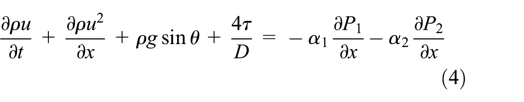
Equation (1) is evolution equation for volume fraction of phase 1, and equations (2), (3), (5), and (6) are conservation of mass and energy for phases 1 and 2, and equation (4) is mixture momentum equation. The term $P_I$ is interfacial pressure. As in a previous study, ¹⁴ interfacial pressure is defined as mixture pressure, and velocity is defined as velocity of the center of mass as in equation (7)

$$P_I={\alpha }_1{P}_1+{\alpha }_2{P}_2$$

(7)

There are still some other closure relations for the interfacial terms, as $P_I=P_1$ and also as in equation (8) based on the model by Furfaro and Saurel^16,19

$$P_I=\frac{Z_1{P}_1+Z_2{P}_2}{Z_1+Z_2}+\mathrm{sign}\left(\frac{\partial {\alpha }_1}{\partial x}\right)\frac{(u_1-u_2)Z_1{Z}_2}{Z_1+Z_2}$$

(8)

The $Z_k$ represents acoustic impedance $Z_k={\rho }_k{c}_k$ . The speed of sound $c_k$ is given in equation (9)

$$c_k^2=\frac{\frac{p_k}{{\rho }_k^2}-{\left(\frac{\partial e}{\partial {\rho }_k}\right)}_{p_k}}{{\left(\frac{\partial e}{\partial p_k}\right)}_{{\rho }_k}},k=1,2$$

(9)

In this article, the closure relation $P_I={\alpha }_1{P}_1+{\alpha }_2{P}_2$ is used for the model of two-phase transient flow. In order to ensure mathematical properties of the model, we take the model in terms of primitive variables as $\partial \varphi /\partial t+B(\partial \varphi /\partial x)=D$ , where the source vector is ${\varphi }^T=[{\alpha }_1,{\rho }_1,{\rho }_2,u,P_1,P_2]$ , and matrix B is given as equation (10)

$$B=\left[\begin{array}{cccccc}u\hfill & \hfill & \hfill & {\alpha }_1\hfill & \hfill & \hfill \\ \multicolumn{1}{c}{}& u\hfill & \hfill & {\rho }_1\hfill & \hfill & \hfill \\ \multicolumn{1}{c}{}& \hfill & u\hfill & {\rho }_2\hfill & \hfill & \hfill \\ \multicolumn{1}{c}{}& \hfill & \hfill & u\hfill & \frac{{\alpha }_1}{\rho }\hfill & \frac{{\alpha }_2}{\rho }\hfill \\ \multicolumn{1}{c}{}& \hfill & \hfill & {\rho }_1{c}_1^2\hfill & u\hfill & \hfill \\ \multicolumn{1}{c}{}& \hfill & \hfill & {\rho }_2{c}_2^2\hfill & \hfill & u\hfill \end{array}\right]$$

(10)

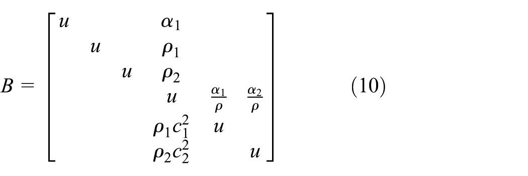
The system is unconditional hyperbolic. As shown in equation (11), there are six eigenvalues in matrix B, four of which are distinct

$${\lambda }_1=u-c{\lambda }_2=u+c{\lambda }_3-{\lambda }_6=u$$

(11)

where c is mixture sound speed which is expressed as $c^2=({\alpha }_1{\rho }_1/\rho )c_1^2+({\alpha }_2{\rho }_2/\rho )c_2^2$ .

Conventional closure relation

EOS

EOS is needed to close the system. A modified form of the stiffened-gas equation of state (SG-EOS) is used with same parameters in Saurel et al. ¹⁹ The stiffened EOS is expressed as equation (12)

$$e_k(p_k,{\rho }_k)=\frac{p_k+{\gamma }_k{\pi }_k}{{\rho }_k({\gamma }_k-1)}+q_k$$

(12)

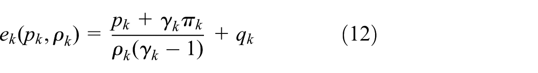
The specific heat ratio ${\gamma }_k$ is given by ${\gamma }_k=C_{p,k}/C_{v,k}$ , and as in the model by Crouzet et al., ¹⁵ ${\pi }_v$ is taken to zero and ${\pi }_l$ is computed as in equation (13)

$${\pi }_l={\rho }_l\left(T_{\mathrm{ref}}\right)({\gamma }_k-1)C_{v,l}{T}_{\mathrm{ref}}-p_{\mathrm{sat}}\left(T_{\mathrm{ref}}\right)$$

(13)

where $T_{\mathrm{ref}}$ is experimental temperature at reference state and $p_{\mathrm{sat}}$ is saturation vapor pressure, shown in equation (14)

$$p_{\mathrm{sat}}=\exp (12.98-\frac{4900}{T_{\mathrm{ref}}})\mathrm{bars}$$

(14)

Interfacial variables

The assumptions on bubble radius we do are as follows:

1. Diameter of bubble is assumed that it develops in a linear growth as the gas volume change as

   $${\alpha }_1=N_g(4/3)\pi R^{3}R=\sqrt[3]{3{\alpha }_{1}n\pi /4}$$

2. Number density per unit volume is assumed as a constant $N_g=a_g{\rho }_g{n}_g$ .

3. There is no deformation in the transient process under the condition of the hypothesis and calculation method of interface area is shown as follows

   $$A_I=4N_g\pi R^2=\frac{3{\alpha }_1}{R}$$

   (15)

Mechanical relaxation rates

Pressure relaxation rates

When dealing with pressure and speed relaxation phenomena under the restriction of many physical conditions, it is reasonable to assume that pressure and speed relaxation time are achieved instantaneously. This assumption is exactly satisfied for interface conditions, when pressure and speed are equalized after each time step on both boundary surfaces. It is regarded that pressure and speed relaxation time are in a microsecond scale, and two characteristics of relaxation time show a positive correlation. The relaxation phenomenon can be approximated to regard as infinitesimal where a larger time step value is selected, ¹³ but for a shorter period, pressure and speed relaxation phenomena have a strong impact on the precision of numerical calculation. The relaxation phenomenon is also related to many parameters of fluid characteristics and changing process.^20,21

Here, for the pressure relaxation phenomenon, the relaxation parameter, as shown in equation, ²² is used (equation (16))

$$\mu =\frac{A_I}{Z_1+Z_2}{Z}_1={\rho }_1{c}_1,Z_2={\rho }_2{c}_2$$

(16)

The mass transfer model

Both air release and water vapor are calculated in the calculation of mass transfer through interface in this work. The gas release process of air and a cavitation model are investigated to improve the overall method in this section. Some improvements are made in the calculation method of mass transfer through the interface based on the method used by Crouzet et al. ¹⁵ to ensure that model is suitable for mass transfer in bubble flow.

It is assumed that mass exchange completes in a very short time, and bubble type is always in a stable state at each time step with mass exchanging as shown in Figure 1, so jump condition through interface is shown in equation (17)

$$\underset{\mathrm{Sg}}{\int }({\rho }_g{Y}_{\mathrm{gi}}{\overrightarrow{u}}_g-{\rho }_g{D}_g\overrightarrow{\nabla }{Y}_{\mathrm{gi}})·{\overrightarrow{n}}_g\mathrm{dS}+\underset{\mathrm{Sl}}{\int }({\rho }_l{Y}_{\mathrm{li}}{\overrightarrow{u}}_l-{\rho }_l{D}_l\overrightarrow{\nabla }{Y}_{\mathrm{li}})·{\overrightarrow{n}}_l\mathrm{dS}=0$$

(17)

Figure 1.

Schematic representation of the mass transfer in a two-fluid control volume.

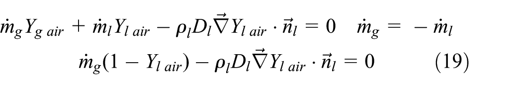
The boundary conditions of air in liquid and gas phases can be written as shown in equation (18)

$$({\rho }_g{Y}_{g\mathrm{air}}{\overrightarrow{u}}_g-{\rho }_g{D}_g\overrightarrow{\nabla }{Y}_{g\mathrm{air}})·{\overrightarrow{n}}_g+({\rho }_l{Y}_{l\mathrm{air}}{\overrightarrow{u}}_l-{\rho }_l{D}_l\overrightarrow{\nabla }{Y}_{l\mathrm{air}})·{\overrightarrow{n}}_l=0$$

(18)

It is assumed that air content in gas phase is 1, that is, gas is pure state. The mass change at the time of boundary conditions is ${\rho }_g{\overrightarrow{u}}_g·{\overrightarrow{n}}_g={\stackrel{·}{m}}_g$ , ${\rho }_l{\overrightarrow{u}}_l·{\overrightarrow{n}}_l={\stackrel{·}{m}}_l$ , and equation (19) is expressed as

$$\begin{array}{c}{\stackrel{·}{m}}_g{Y}_{g\mathrm{air}}+{\stackrel{·}{m}}_l{Y}_{l\mathrm{air}}-{\rho }_l{D}_l\overrightarrow{\nabla }{Y}_{l\mathrm{air}}·{\overrightarrow{n}}_l=0{\stackrel{·}{m}}_g=-{\stackrel{·}{m}}_l{\stackrel{·}{m}}_g(1-Y_{l\mathrm{air}})-{\rho }_l{D}_l\overrightarrow{\nabla }{Y}_{l\mathrm{air}}·{\overrightarrow{n}}_l=0\hfill \end{array}$$

(19)

Fick’s first law describes the change of concentration of dissolved gas in liquid, as shown in equation (20)

$$J_{l,\mathrm{air}}=-{\rho }_l{D}_l\overrightarrow{\nabla }{Y}_{l\mathrm{air}}={\rho }_{l}k(Y_{l\mathrm{air}I}-Y_{l\mathrm{air}\infty })·{\overrightarrow{n}}_l$$

(20)

Then mass flux rate per unit area can be expressed as shown in equation (21)

$${\stackrel{·}{m}}_g=\frac{(Y_{l\mathrm{air}I}-Y_{l{\mathrm{air}}_{\infty }}){\rho }_{l}k}{Y_{l\mathrm{air}I}-1}$$

(21)

The quality of gas release rate equation can be expressed in corresponding to Henry’s law. The mass flux rate per unit area can be expressed as shown in equation (22), when combined with $M{Y}_{l\mathrm{air}i}=P_i/\mathrm{He}$

$${\stackrel{·}{m}}_g=\frac{(P_I-P_{\infty }){\rho }_{l}k}{(P_I-\mathrm{HeM})}$$

(22)

where $Y_{l\mathrm{air}I}$ represents the concentration of air in liquid at interface, $Y_{l\mathrm{air}\infty }$ represents the concentration of air in liquid far from interface, M represents molar mass, He represents Henry coefficients, k represents spread coefficient, and $D_k$ represents mass diffusivity of air in water.

The spread coefficient k is expressed according to definition in Sherwood number, as shown in equation (23)

$$\{\begin{array}{c}\mathrm{Sh}=2+0.95R{e}^{0.5}S{c}^{1/3}2<\mathrm{Re}<2000\hfill \\ \multicolumn{1}{c}{\mathrm{Sh}=0.347R{e}^{0.62}S{c}^{1/3}2000<\mathrm{Re}<17,000}\end{array}$$

(23)

where the Sherwood number is $\mathrm{Sh}=\mathrm{kd}/D_k$ , the Reynolds number is $\mathrm{Re}=\mathrm{ud}\rho /\mu$ , and the Schmidt number is $\mathrm{Sc}=\mu /\rho D_k$ .

The method of cavitation calculation in liquid–vapor mass transfer

The cavitation model is introduced from calculation of interface mass transfer. It will produce a cavitation phenomenon when pressure is lower than saturated evaporation pressure. It is assumed that production of the vapor during cavitation does not influence the bubble production from the gas phase in air produce, that is, they are regarded as two different processes; however, both of them lead to the change in gas phase volume fraction.

When pressure drops to saturated evaporation pressure, according to the Rayleigh–Plesset Model under the zero gravity, cavitation is calculated in a control volume. The calculation is divided into two parts: evaporation and condensation. Assuming no heat transfer, mass transfer is therefore caused only by change of pressure, and its condensation is slower than its transpiration,^23,24 which can be expressed as shown in equation (24)

$${\stackrel{·}{m}}_{\mathrm{fg}}=F_{\mathrm{vap}}\frac{3r_{\mathrm{nuc}}(1-r_g){\rho }_g}{R_{\mathrm{nuc}}}\sqrt{\frac{2|p_v-p|}{{\rho }_f}}\mathrm{sgn}(p_v-p)$$

(24)

$${\stackrel{·}{m}}_{\mathrm{fg}}=F_{\mathrm{cond}}\frac{3r_g{\rho }_g}{R_B}\sqrt{\frac{2|p_v-p|}{{\rho }_f}}\mathrm{sgn}(p_v-p)$$

(25)

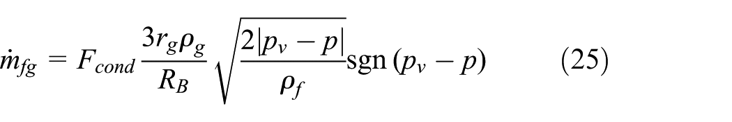
where $F_{\mathrm{vap}}=50$ , $F_{\mathrm{cond}}=0.01$ , $p=p_{\mathrm{sat}}$ , and $r_{\mathrm{nuc}}$ is the volume fraction of non-condensable gas.

Numerical resolution

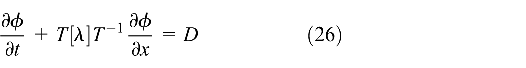
The control equation (26) is expressed by FVS as follows

$$\frac{\partial \varphi }{\partial t}+T\left[\lambda \right]T^{-1}\frac{\partial \varphi }{\partial x}=D$$

(26)

The eigenvalues of matrix are divided into two parts ( ${\lambda }^{+}$ and ${\lambda }^{-}$ ), then the control equation can be expressed as shown below

$$\begin{array}{c}\frac{\partial \varphi }{\partial t}+F^{+}\frac{\partial \varphi }{\partial x}+F^{-}\frac{\partial \varphi }{\partial x}=D\hfill \\ F^{+}=T\left[{\lambda }^{+}\right]T^{-1},F^{-}=T\left[{\lambda }^{-}\right]T^{-1}\hfill \end{array}$$

Hence, finite difference method is used to solve gas–liquid two-phase flow equations by combining FVS method of Steger–Warming with the NND scheme.

NND, proposed by Zhang and Zhuang, ²⁵ is a non-oscillatory, containing, no free parameters and dissipative scheme. This scheme can effectively suppress the numerical oscillation in calculation using different difference scheme in upstream and downstream of the shock wave areas. It has a very high resolution in capturing the shock wave and a clear physical meaning with second-order accuracy in space. The explicit scheme is shown as equations (27) and (28)

$$U_j^{n+1}=U_j^n-\frac{\Delta t}{\Delta x}\left\{\begin{array}{l}{F}_j^{+}{U}_j^n+\frac{1}{2}\min \mathrm{mod}\left(\Delta F_{j-\frac{1}{2}}^{+}{U}_{j-\frac{1}{2}}^n,\Delta F_{j+\frac{1}{2}}^{+}{U}_{j+\frac{1}{2}}^n\right)\\ +F_{j+1}^{-}{U}_{j+1}^n-\frac{1}{2}\min \mathrm{mod}\left(\Delta F_{j+\frac{1}{2}}^{-}{U}_{j+\frac{1}{2}}^n,\Delta F_{j+\frac{3}{2}}^{-}{U}_{j+\frac{3}{2}}^n\right)\\ -F_{j-1}^{+}{U}_{j-1}^n-\frac{1}{2}\min \mathrm{mod}\left(\Delta F_{j-\frac{3}{2}}^{+}{U}_{j-\frac{3}{2}}^n,\Delta F_{j-\frac{1}{2}}^{+}{U}_{j-\frac{1}{2}}^n\right)\\ -F_j^{-}{U}_j^n+\frac{1}{2}\min \mathrm{mod}\left(\Delta F_{j-\frac{1}{2}}^{-}{U}_{j-\frac{1}{2}}^n,\Delta F_{j+\frac{1}{2}}^{-}{U}_{j+\frac{1}{2}}^n\right)\end{array}\right\}$$

(27)

where F is a function of U

$$\begin{array}{c}\Delta F_{j-\frac{1}{2}}^{\pm }=F_j^{\pm }-F_{j-1}^{\pm }\hfill \\ \Delta F_{j+\frac{1}{2}}^{\pm }=F_{j+1}^{\pm }-F_j^{\pm }\hfill \\ \Delta F_{j+\frac{3}{2}}^{\pm }=F_{j+2}^{\pm }-F_{j+1}^{\pm }\hfill \\ \Delta F_{j-\frac{3}{2}}^{\pm }=F_{j-1}^{\pm }-F_{j-2}^{\pm }\hfill \end{array}$$

$$minmod(x,y)=\{\begin{array}{cc}0\hfill & \mathrm{xy}<0\hfill \\ \multicolumn{1}{c}{\mathrm{sign}(x)•min(\left|x\right|,\left|y\right|)}& \mathrm{xy}\ge 0\hfill \end{array}$$

(28)

The Steger–Warming FVS method combined with NND scheme

The derivative of positive and negative flux at zero eigenvalue is discontinuous using the Steger–Warming FVS method. The derivative discontinuation in flux will produce oscillations near zero eigenvalue, which would affect the precision and stability of the numerical calculation. Hence, flux derivative discontinuity should be considered in calculation by Steger–Warming FVS. Therefore, the Steger–Warming FVS combined with NND is as shown in equation (29)

$${\Phi }_j^{n+1}={\Phi }_j^n+\Delta tE-\frac{\Delta t}{\Delta z}\left[\begin{array}{l}{F}_j^{+}{\Phi }_j^n+\frac{1}{2}\min \mathrm{mod}\left(\Delta F_{j-\frac{1}{2}}^{+}{\Phi }_{j-\frac{1}{2}}^n,\Delta F_{j+\frac{1}{2}}^{+}{\Phi }_{j+\frac{1}{2}}^n\right)\\ +F_{j+1}^{-}{\Phi }_{j+1}^n-\frac{1}{2}\min \mathrm{mod}\left(\Delta F_{j+\frac{1}{2}}^{-}{\Phi }_{j+\frac{1}{2}}^n,\Delta F_{j+\frac{3}{2}}^{-}{\Phi }_{j+\frac{3}{2}}^n\right)\\ -F_{j-1}^{+}{\Phi }_{j-1}^n-\frac{1}{2}\min \mathrm{mod}\left(\Delta F_{j-\frac{3}{2}}^{+}{\Phi }_{j-\frac{3}{2}}^n,\Delta F_{j-\frac{1}{2}}^{+}{\Phi }_{j-\frac{1}{2}}^n\right)\\ -F_j^{-}{\Phi }_j^n+\frac{1}{2}\min \mathrm{mod}\left(\Delta F_{j-\frac{1}{2}}^{-}{\Phi }_{j-\frac{1}{2}}^n,\Delta F_{j+\frac{1}{2}}^{-}{\Phi }_{j+\frac{1}{2}}^n\right)\end{array}\right]$$

(29)

Boundary condition

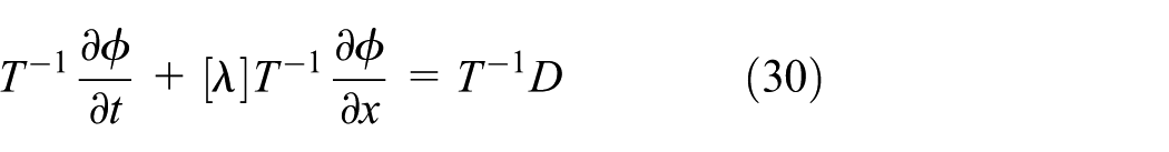
The boundary condition is described as shown in equation (30)

$$T^{-1}\frac{\partial \varphi }{\partial t}+\left[\lambda \right]T^{-1}\frac{\partial \varphi }{\partial x}=T^{-1}D$$

(30)

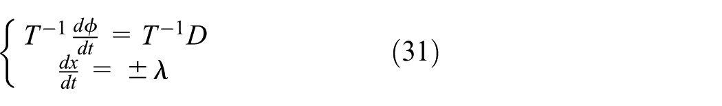
The method of characteristic is chosen to determine boundary conditions, as shown in equation (31)

$$\{\begin{array}{c}{T}^{-1}\frac{d\varphi }{\mathrm{dt}}=T^{-1}D\hfill \\ \multicolumn{1}{c}{\frac{\mathrm{dx}}{\mathrm{dt}}=\pm \lambda }\end{array}$$

(31)

Left eigenvectors for original matrix B are as follows in equations (32) and (33)

$${\varphi }^T=[{\alpha }_1,{\rho }_1,{\rho }_2,u,P_1,P_2]$$

(32)

$$T^{-1}=\left\{\begin{array}{cccccc}\hfill & \hfill & \hfill & -\frac{{\rho }_2{c}_2^2}{2c}\hfill & \frac{{\alpha }_1{\rho }_2{c}_2^2}{2\rho c^2}\hfill & \frac{{\alpha }_2{\rho }_2{c}_2^2}{2\rho c^2}\hfill \\ \multicolumn{1}{c}{}& \hfill & \hfill & \frac{{\rho }_2{c}_2^2}{2c}\hfill & \frac{{\alpha }_1{\rho }_2{c}_2^2}{2\rho c^2}\hfill & \frac{{\alpha }_2{\rho }_2{c}_2^2}{2\rho c^2}\hfill \\ \multicolumn{1}{c}{1}& \hfill & \hfill & \hfill & -\frac{{\alpha }_1^2}{\rho c^2}\hfill & -\frac{{\alpha }_1{\alpha }_2}{\rho c^2}\hfill \\ \multicolumn{1}{c}{}& 1\hfill & \hfill & \hfill & -\frac{{\alpha }_1{\rho }_1}{\rho c^2}\hfill & -\frac{{\alpha }_2{\rho }_1}{\rho c^2}\hfill \\ \multicolumn{1}{c}{}& \hfill & 1\hfill & \hfill & -\frac{{\alpha }_1{\rho }_2}{\rho c^2}\hfill & -\frac{{\alpha }_2{\rho }_2}{\rho c^2}\hfill \\ \multicolumn{1}{c}{}& \hfill & \hfill & \hfill & -\frac{{\alpha }_1{\rho }_2{c}_2^2}{\rho c^2}\hfill & \frac{{\alpha }_1{\rho }_1{c}_1^2}{\rho c^2}\hfill \end{array}\right\}$$

(33)

The corresponding change parameters are required to be calculated using boundary conditions from left eigenvectors. Other conditions in upstream and downstream can be determined subsequently. The compatibility equations are shown in equation (34)

$$\begin{array}{c}{\varphi }_R={\varphi }_C+\frac{\Delta t}{\Delta x}(c-u)({\varphi }_C-{\varphi }_B)\hfill \\ {\varphi }_L={\varphi }_C-\frac{\Delta t}{\Delta x}(c+u)({\varphi }_C-{\varphi }_A)\hfill \\ {\varphi }_L={\varphi }_C-\frac{\Delta t}{\Delta x}(u)({\varphi }_C-{\varphi }_A)\hfill \end{array}$$

(34)

Computation examples and validation

Simpson’s valve closure water hammer experiment

Simpson’s valve closure water hammer experiment is chosen to compare to the simulations, which has been already analyzed in the literature. ¹⁵ The analysis data from Simpson ²⁶ are selected for calculation and comparison. The experiment consists of a horizontal pipe (which has 1 m high slope), upstream tank, and downstream valve. The fluid pressure is measured at three points along the 36 m pipeline which are located at 36, 27, and 9 m. The main parameters of fluid are referenced to the literature, ¹⁵ and the specific data are listed in Tables 1 and 2 as shown below. The number density per unit volume is N_g = 2 × 10⁶ empirically. Computing time step is 5 × 10⁻⁵ s. The water and air density is 998.2 and 2.52 kg/m³, respectively, and liquid water vapor density value is 1 kg/m³. The saturation vapor pressure is 2237 Pa.

Table 1.

The initial conditions of Simpson’s experiment.

	Before tank	Tank
a 1	10−6	10−6
P 1 P 2	33.63 m	33.63 m
U 1 U 2	0.401 m/s	0.401 m/s
hf	0.45 m	0.45 m

Table 2.

EOS parameters for liquid and vapor water for Simpson’s experiment.

Phase	π (Pa)	Cp	Cv	γ	q
Liquid	6.928 × 108	4183	1840.48	2.27	−1.14 × 106
Gas	0	1800	1344.06	1.34	2.01 × 106

EOS: equation of state.

The speed is set as the boundary condition for the calculation as shown in Figure 2, where the interval velocity between 1173 and 1424 ms is used to forecast mixed pressure changes at different points. As seen in Figure 2, there is a good agreement between the simulation and experimental value in the result of mixed pressure, with a slight deviation only at peak pressure, but they still follow the same trend in the pressure. In addition, if the pressure is inputted as the boundary conditions, the prediction of the transient pressure would be improved greatly.

Figure 2.

The pressure $P_I$ versus time at different positions in Simpson’s hammer experiment: comparison between the model and the experiments: (a) the comparison of pressure at Z = 9 m, (b) the comparison of pressure at Z = 27 m, and (c) the comparison of pressure at Z = 36 m.

The simulation of the power failure in pump system

In order to simulate pressure and volume fraction change in the pipeline at power failure of pump system, comparison experiments are performed for the simulation in the Key Lab of Hydraulic Machinery Transient, MOE, in Wuhan University. The experiment system diagram is shown in Figure 3. The system is set composed of a water tank, a pump, valves, and long horizontal pipeline. The total length of pipeline is 600 m, the diameter is 0.1 m, the material of tube is galvanized steel, the thickness of the pipe is about 3–4 mm, the sound speed is about 1280 m/s, and water level of the constant water tank is 2.3 m. The gate valve and multifunctional pump-control valve are parallel in this system, which can be used in different experiments. The position of P0 (0 m), P1 (100 m), and P2 (555 m) after valve position are data collection points on the pipeline.

Figure 3.

The sketch of the experiment.

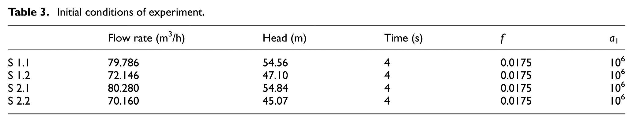
Two schemes are proposed for the experiments: scheme 1 (S1), no valve is closed when the power was cut off (which the fluid flows freely in tube); and scheme 2 (S2), the multifunctional pump-control valve is used when the power was cut off (the bypass valve is closed). Experimental parameters are shown in Table 3.

Table 3.

Initial conditions of experiment.

	Flow rate (m3/h)	Head (m)	Time (s)	f	a 1
S 1.1	79.786	54.56	4	0.0175	106
S 1.2	72.146	47.10	4	0.0175	106
S 2.1	80.280	54.84	4	0.0175	106
S 2.2	70.160	45.07	4	0.0175	106

Thermodynamic parameters of phase can be referred in the literature. ²⁶ In reference to sound speed under premise of its parameters, the parameters can be identified as shown in Table 4. The number density per unit volume is also taken as N_g = 2 × 10³ empirically. Computing time step is 5 × 10⁻⁵ s. The water and air density value is 998.2 and 2.52 kg/m³, respectively, while liquid water vapor density value is 1 kg/m³. The saturation vapor pressure is 2237 Pa. In this calculation, the pressure is inputted as boundary conditions, and the following four experiments and calculation are compiled in Figures 5–7.

Table 4.

EOS parameters for liquid and vapor water for the experiment.

Phase	π (Pa)	Cp	Cv	γ	q
Liquid	7.228 × 108	4178	1840.48	2.27	−1.14 × 106
Gas	0	1841	1344.06	1.37	2.03 × 106

EOS: equation of state.

Figure 4 shows the absolute pressure and void fraction change at P1 and P2 points in scheme 1.1. The experimental value of pressure wave attenuation is faster than the theoretical one due to the knee joints in the system. Hence, the energy loss coefficient is used to mathematically compare the results, which combined with the friction coefficient and temporarily set as 3.0. The experimental values and calculated values are shown in Figure 4. A reasonable agreement is achieved upon comparison.

Figure 4.

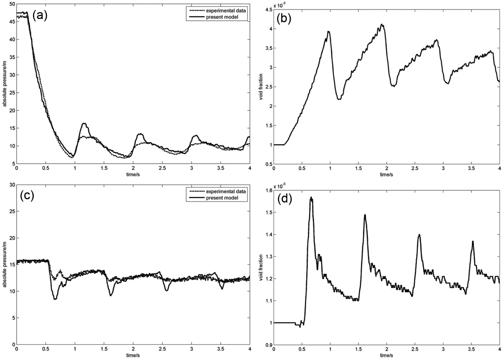
Comparison between the experimental results and computed S 1.1: (a) the comparison of pressure at Z = 100 m, (b) the calculation of void fraction at Z = 100 m, (c) the comparison of pressure at Z = 555 m, and (d) the calculation of void fraction at Z = 555 m.

Figure 5 shows absolute pressure and void fraction change at P1 and P2 points in scheme 1.2. Due to the reduction in flow rate, the energy loss coefficient is defined as 2.5.

Figure 5.

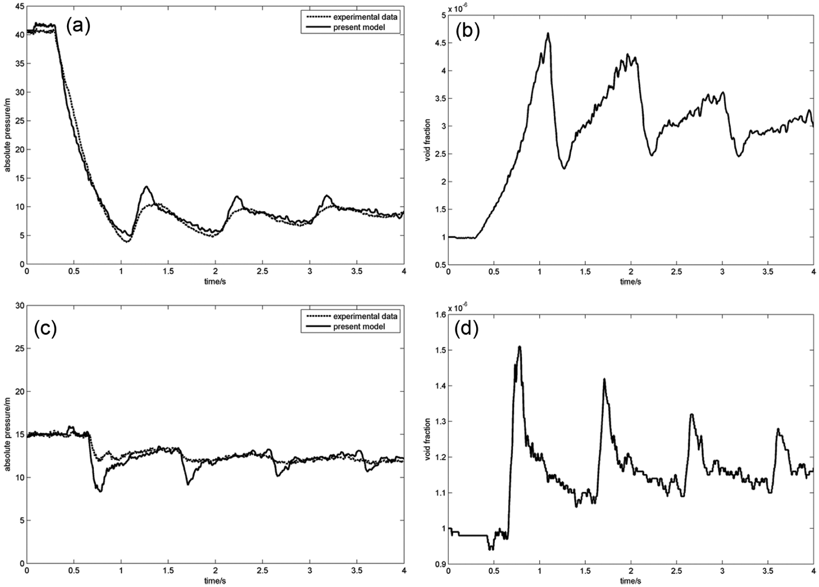
Comparison between the experimental results and computed S 1.2: (a) the comparison of pressure at Z = 100 m, (b) the calculation of void fraction at Z = 100 m, (c) the comparison of pressure at Z = 555 m, and (d) the calculation of void fraction at Z = 555 m.

Figure 6 shows the absolute pressure and void fraction change at P1 and P2 points in scheme 2.1.

Figure 6.

Comparison between the experimental results and computed S 2.1: (a) the comparison of pressure at Z = 100 m, (b) the calculation of void fraction at Z = 100 m, (c) the comparison of pressure at Z = 555 m, and (d) the calculation of void fraction at Z = 555 m.

Figure 7 shows absolute pressure and void fraction change at P1 and P2 points in scheme 2.2. The comparison of the pressure curves show that this gas–liquid two-phase flow method can predict one-dimensional two-phase transient flow well, as well as for a good forecast analysis of void fraction at different section. It has a certain practical significance in industrial pipe system to the two-phase flow.

Figure 7.

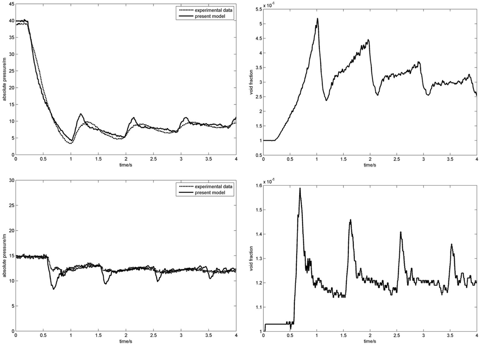
Comparison between the experimental results and computed S 2.2: (a) the comparison of pressure at Z = 100 m, (b) the calculation of void fraction at Z = 100 m, (c) the comparison of pressure at Z = 555 m, and (d) the calculation of void fraction at Z = 555 m.

Conclusion

In this article, the two-fluid model for the conservation equation is calculated with mass transfer in gas–liquid two-phase transient flow using Steger–Warming FVS method which is combined with an NND scheme. By comparing the experiment and numerical computation, the following conclusions are reached:

1. The combination of the Steger–Warming FVS and NND difference method in conservation gas–liquid two-phase flow equations can have a very good guarantee in stability of the simulation.

2. The equation of mass transfer is deduced by concentration change in two-phase flow, and this formula has great significance in industrial application, especially in bubble two-phase flow in pipelines.

3. A reasonable agreement is achieved by comparing the results between experimental and simulation. This method is proved to be capable of capturing shock waves and interface mass exchange during the transient process in bubble flow while suppressing the oscillation problem in the pipeline from the calculation simultaneously.

However, this model also has some certain insufficiencies due to the introduction of assumptions: (1) number density per unit volume is assumed to not change, (2) the fragmentation and integration of the bubbles are ignored, (3) no transformation in the flow model occurred, and (4) the fluid–structure interaction process is ignored. Those problems are currently being investigated to improve the model in the future.