Sage Journals: Discover world-class research

Abstract

In order to realize the nonlinear dynamic decoupling control of a 5-degree-of-freedom bearingless induction motor which consists of a 3-degree-of-freedom magnetic bearing and a 2-degree-of-freedom bearingless induction motor, a decoupling control strategy based on least squares support vector machine inverse is proposed. First, on the basis of introducing the structure of 5-degree-of-freedom bearingless induction motor, the mathematical model is derived. At the same time, the reversibility of the mathematical model is analyzed. Second, the inverse model of 5-degree-of-freedom bearingless induction motor is identified using the regress capability for high-dimensional nonlinear least squares support vector machine within limited samples. In addition, the particle swarm optimization algorithm is used to optimize parameters of the least squares support vector machine, which improves the fitting and predictive precision of the model. Third, combining the least squares support vector machine inverse model with the original system constitutes the pseudo linear system and then proportional–integral–derivative closed-loop controllers are designed to realize the compound control for the 5-degree-of-freedom bearingless induction motor system. The dynamic decoupling control among the radial and axial displacements, speed, and flux linkage is achieved. The simulation and preliminary experiment results all verify the effectiveness of the proposed control strategy.

Keywords

5-Degree-of-freedom bearingless induction motor magnetic bearing least squares support vector machine inverse inverse model decoupling control

Introduction

Bearingless induction motor (BIM), with the characteristics of magnetic bearing and traditional induction motor, has the advantages of nonabrasion, nonlubrication, simple structure, high mechanical strength, reliable and robust, low cogging torque ripple, and wide range of weak magnetic. It can realize the unsupported operation in high or ultra high speed. It has a broad application prospect in the field of special electrical transmission/driver, such as high-speed turbo molecular pump, high-speed and high-precision numerical control machine tool, high-speed centrifugal, agricultural robots, flywheel energy storage, and so on.^1–5

At present, the research on BIM is mainly concentrated on the 2-degree-of-freedom (DOF) BIM, which is a kind of 2-DOF radial levitation system.^6–9 Using a conventional self-aligning ball bearing supporting one end of the rotating shaft, 2-DOF BIM can only carry out the radial levitation experiment, and the axial levitation movement experiment cannot be realized. Therefore, this motor does not realize the complete nonbearingless. Instead of the conventional self-aligning ball bearing, the 3-DOF radial–axial hybrid magnetic bearing (RAHMB)^10–12 is used in the 5-DOF BIM and the suspension control in axial DOF, and another two radial DOFs on the end of the shaft are carried out, which realizes the complete suspension control of the shaft. Therefore, it has important scientific significance and practical application value to research the 5-DOF BIM.

With complex electromagnetic relationship, 5-DOF BIM is a multi-variable, nonlinear, strong coupling time-varying system. Strong coupling exists not only between the motor torque subsystem and the rotor flux subsystem but also between radial and axial suspension force subsystems. Thus, the nonlinear dynamic decoupling control for 5-DOF BIM is necessary to realize the stable suspension of rotor and achieve stepless speed regulation under different working conditions. With the clear physical conception and simple mathematical deduction, the inverse system method has become one of the effective ways to achieve decoupling of bearingless motor system. On one hand, it provides people a comprehensive understanding of the control theory of bearingless motor system. On the other hand, it provides good theoretical basis for advanced and practical control strategy. But the inverse system model is hard to accurately obtain in engineering practice.^13–15 Using the nonlinear approximation ability of neural network, neural network inverse system method can identify BIM inverse model and solve the tough problem of obtaining the accurate inverse system model, but the neural network’s own defects (local minimum, complex computation, over learning, structure type choice over relying on experience, etc.) limit the further application of the neural network inverse system method.^12,16,17 Support vector machine (SVM) inverse method is a kind of nonlinear control strategy by combining the inverse system theory with SVM. Using the SVM as a general identification model of inverse system and the vector relative order of the known system, it can obtain SVM α-order inverse system through the right training. The least squares support vector machine (LSSVM) that was proposed by Suykens and Vandewalle is an extension of SVM, which turns the inequality constraints of the SVM into equality constraints and only needs to solve a linear equation. In addition, using the learning rules of structural risk minimization, the LSSVM has overcome the defects of the learning rule of empirical risk minimization of neural network.¹⁸ It has the advantages of stable topology structure, fast training speed, and small sample learning ability, without the problems of local minimum and dimension disaster. It has been widely used in identification and control of linear or nonlinear system in recent years.^19–21

Taking the 5-DOF BIM as the research object, combining the regression ability of nonlinear function of the LSSVM and the linear decoupling characteristics of traditional analysis inverse system method, this article proposes the least squares support vector machine inverse (LSSVMI) decoupling control strategy of 5-DOF BIM. On the basis of introducing the structure and working principle of 5-DOF BIM, this article analyzes the existence of 5-DOF BIM inverse system. At the same time, the LSSVM is used to identify the inverse model of 5-DOF BIM. The particle swarm optimization (PSO) algorithm is adopted to acquire the optimization parameter of LSSVM^22–26 which improves the fitting and forecast precision of the inverse model. Taking the LSSVMI model as the feed-forward controller of the original system and the proportional–integral–derivative (PID) controller as a feedback controller, the compound control for the 5-DOF BIM is conducted, which realizes the dynamic nonlinear decoupling control between speed, flux, axial displacement, and radial displacement. Finally, the simulation and the preliminary experiments verify the correctness and effectiveness of the proposed control strategy.

Basic structure and mathematics model of 5-DOF BIM

The 5-DOF BIM consists of the units of 3-DOF RAHMB and 2-DOF BIM. Due to the 3-DOF RAHMB replacing the conventional self-aligning ball bearing, the 5-DOF BIM implements the suspension control of an axial DOF and the other two radial DOFs on the end of the shaft. Consequently, the rotor has been effectively suspended in five DOF positions and realizes the completely bearingless of the BIM. The structure diagram of 5-DOF BIM is shown in Figure 1.

Figure 1.

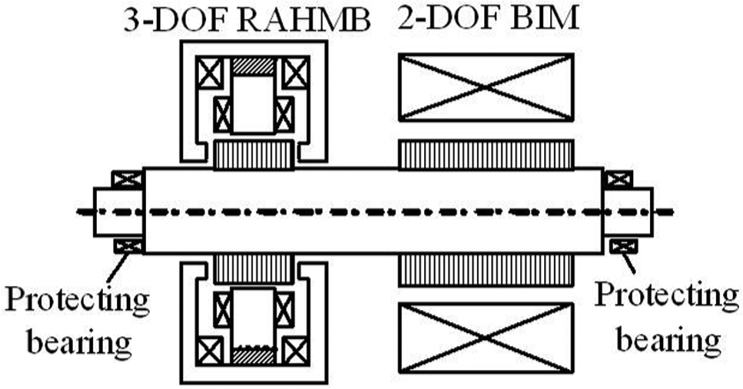
Structure diagram and physical diagram of 5-DOF BIM.

The structure diagram of 3-DOF RAHMB is shown in Figure 2. The 3-DOF RAHMB consists of radial control coil, 3-pole radial stator, axial control coil, axial stator, permanent magnet, and rotor. The permanent magnet is made from the rare earth permanent magnet material NdFeB, and the iron core of radial stator is composed of stacked silicon steel sheet. For the 3-DOF RAHMB, the radial adopts alternating current (AC) excitation and the axial adopts direct current (DC) excitation, and the radial magnetized permanent magnet provides the bias flux of the axial–radial. Therefore, with the characteristics of permanent magnet bias and AC excitation, the 3-DOF RAHMB has the advantages of compact structure, high efficiency, flexible control, low cost, low loss, and so on.

Figure 2.

Structure diagram of 3-DOF RAHMB.

When the 3-DOF RAHMB works, the three coils (A, B, and C) of 3-pole radial stator are evenly distributed along the circumference by 120°. The two radial DOFs are controlled by adjusting the compound rotating magnetic field produced by the three-phase AC in the three coils, and the single axial DOF is controlled by the two axial coils in the axial stator. When the 3-DOF RAHMB is suspended steadily, the static biased magnetic field generated by the permanent magnet makes the rotor in the reference balance position.

Mathematical model of 3-DOF RAHMB radial–axial suspension force

Using the subscript l expresses the related variables of 3-DOF RAHMB; x_l, y_l, and z_l represent the displacement in radial x and y and axial z of the rotor of 3-DOF RAHMB, respectively; i_lx, i_ly, and i_lz represent the corresponding control current of the radial x and y and axial z, respectively. According to the equivalent magnetic circuit method and virtual displacement theorem, the radial–axial levitation force of the 3-DOF RAHMB can be shown as follows⁸

{\begin{matrix} F_{lx} = \frac{3}{2} k_{xy} \cdot x_{l} + \sqrt{\frac{3}{2}} k_{ixy} \cdot i_{lx} \\ F_{ly} = \frac{3}{2} k_{xy} \cdot y_{l} + \sqrt{\frac{3}{2}} k_{ixy} \cdot i_{ly} \\ F_{lz} = k_{z} \cdot z_{l} + k_{iz} \cdot i_{lz} \end{matrix}

(1)

where F_lx, F_ly, and F_lz are the suspension forces of radial x and y and axial z, respectively; k_xy and k_ixy are the radial force/the displacement stiffness and displacement force/the current stiffness of 3-DOF RAHMB, respectively; and k_z and k_iz are the axial force/the displacement stiffness and displacement force/the current stiffness of 3-DOF RAHMB, respectively; the specific equations can be shown as follows

{\begin{matrix} k_{xy} = \frac{μ_{0} \cdot F_{m}^{2}}{9 {(\frac{δ_{a}}{2 S_{a}} + \frac{δ_{r}}{3 S_{r}})}^{2} S_{r} δ_{r}} \\ k_{ixy} = \frac{(\frac{δ_{a}}{S_{a}} + \frac{δ_{r}}{S_{r}}) μ_{0} \cdot F_{m} N_{r}}{9 {(\frac{δ_{a}}{2 S_{a}} + \frac{δ_{r}}{3 S_{r}})}^{2} δ_{r}} - \frac{μ_{0} \cdot F_{m} N_{r} δ_{a}}{18 {(\frac{δ_{a}}{2 S_{a}} + \frac{δ_{r}}{3 S_{r}})}^{2} S_{a} δ_{r}} \\ k_{z} = \frac{μ_{0} \cdot F_{m}^{2}}{2 {(\frac{δ_{a}}{2 S_{a}} + \frac{δ_{r}}{3 S_{r}})}^{2} δ_{a} S_{a}} \\ k_{iz} = - \frac{μ_{0} \cdot F_{m} \cdot N_{z}}{2 (\frac{δ_{a}}{2 S_{a}} + \frac{δ_{r}}{3 S_{r}}) δ_{a}} \end{matrix}

(2)

where F_m is the magnetic motive force of permanent magnet; µ₀ is the permeability of vacuum; N_r and N_z are the turns of the radial and axial control coil, respectively; S_r and S_a are the magnetic pole areas of radial and axial, respectively; and δ_r and δ_a are the air-gap lengths of radial and axial, respectively.

Mathematical model of 2-DOF BIM

BIM is a new type of motor which breaks through the traditional motor theory of keeping the balance of air-gap magnetic field to produce electromagnetic torque. Using the structure similarity between the magnetic bearing and motor stator, BIM is formed by embedding another radial levitation force windings based on the existing windings in the stator of ordinary induction motor. Through adjusting the current in the radial levitation force windings, the symmetry of air-gap magnetic field is destroyed and thus produces torque and suspension force so as to realize the suspension and rotation functions.

Using the subscript r expresses the related variables of 2-DOF BIM. The virtual displacement method is adopted to deduct the radial suspension model of 2-DOF BIM. The inductance matrix [L] is shown as follows²

[L] = [\begin{matrix} L_{1 s} & 0 & - M x_{r} & M y_{r} \\ 0 & L_{1 s} & M y_{r} & M x_{r} \\ - M x_{r} & M y_{r} & L_{2 s} & 0 \\ M y_{r} & M x_{r} & 0 & L_{2 s} \end{matrix}]

(3)

where the torque winding self-induction L_1s and suspension force winding self-induction L_2s are constants; x_r and y_r are the radial displacements in the directions of x and y of the 2-DOF BIM rotor, respectively; and M is the mutual inductance of the two sets of winding. According to the relationship of energy conversion, the equation of magnetic energy storage by 2-DOF BIM can be written as follows

W_{m} = \frac{1}{2} {[i]}^{T} [L] [i]

(4)

where the current matrix is $[i] = [\begin{matrix} i_{d 1 s} & i_{q 1 s} & i_{d 2 s} & i_{q 2 s} \end{matrix}]^{T}$ and i_d_1s, i_q_1s, i_d_2s, and i_q_2s are the components of torque winding and suspension winding current in d–q axis, respectively.

Substituting formula (3) into formula (4), the following can be obtained

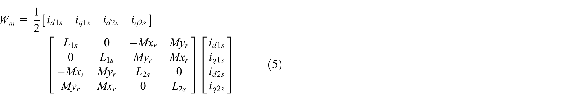
W_{m} = \frac{1}{2} [\begin{matrix} i_{d 1 s} & i_{q 1 s} & i_{d 2 s} & i_{q 2 s} \end{matrix}] [\begin{matrix} L_{1 s} & 0 & - M x_{r} & M y_{r} \\ 0 & L_{1 s} & M y_{r} & M x_{r} \\ - M x_{r} & M y_{r} & L_{2 s} & 0 \\ M y_{r} & M x_{r} & 0 & L_{2 s} \end{matrix}] [\begin{matrix} i_{d 1 s} \\ i_{q 1 s} \\ i_{d 2 s} \\ i_{q 2 s} \end{matrix}]

(5)

According to the virtual displacement principle, the suspension force model of the 2-DOF BIM is as follows²¹

[\begin{matrix} {F_{r}}_{x} \\ F_{ry} \end{matrix}] = [\begin{matrix} \frac{\partial W_{m}}{\partial x_{r}} \\ \frac{\partial W_{m}}{\partial y_{r}} \end{matrix}] = M [\begin{matrix} - i_{d 1 s} & i_{q 1 s} \\ i_{q 1 s} & i_{d 1 s} \end{matrix}] [\begin{matrix} i_{d 2 s} \\ i_{q 2 s} \end{matrix}]

(6)

The electromagnetic torque T_e of 2-DOF BIM in the synchronous rotating coordinate d–q can be shown as follows¹

T_{e} = P_{1} \frac{L_{m 1 r}}{T_{r}} (ψ_{dr} i_{q 1 s} - ψ_{qr} i_{d 1 s})

(7)

where P₁ is the number of pole-pairs of torque winding; T_r is a constant of rotor time; L_m_1r is the mutual inductance between torque winding and rotor; and ψ_dr and ψ_qr are the components of rotor flux in d–q-axis, respectively.

Mathematical model of 5-DOF BIM

Figure 3 shows the stress analysis diagram of rigid rotor for the 5-DOF BIM. In this diagram, the coordinate origin o represents the center of mass; x, y, and z are the coordinate axes of the rotor; m is the mass of the rotor; ω is the angular velocity of rotor; J is the rotational inertia; T_L is the load torque; and f_lx, f_ly, fl_z, f_rx, and f_ry are the outside disturbances in the x_l, y_l, z_l, x_r, and y_r directions, respectively. The equations of motion of the system can be obtained from the rotor dynamics theory as follows

{\begin{matrix} m {\overset{\cdot\cdot}{x}}_{l} = f_{lx} - F_{lx} \\ m {\overset{\cdot\cdot}{y}}_{l} = f_{ly} - F_{ly} \\ m {\overset{\cdot\cdot}{z}}_{l} = f_{lz} - F_{lz} \\ m {\overset{\cdot\cdot}{x}}_{r} = f_{rx} - F_{rx} \\ m {\overset{\cdot\cdot}{y}}_{r} = f_{ry} - F_{ry} \\ \frac{J}{P_{1}} \overset{\cdot}{ω} = T_{e} - T_{L} \end{matrix}

(8)

Figure 3.

Rotor stress analysis diagram.

The state variables are selected as follows

X = [x_{1}, x_{2}, \dots, x_{12}, x_{13}]^{T} = {[x_{l}, y_{l}, z_{l}, x_{r}, y_{r}, {\overset{\cdot}{x}}_{l}, {\overset{\cdot}{y}}_{l}, {\overset{\cdot}{z}}_{l}, {\overset{\cdot}{x}}_{r}, {\overset{\cdot}{y}}_{r}, ω, ψ_{dr}, ψ_{qr}]}^{T}

(9)

The input variables are as follows

U = {[u_{1}, u_{2}, \dots, u_{6}, u_{7}]}^{T} = {[i_{lx}, i_{ly}, i_{lz}, i_{d 1 s}, i_{q 1 s}, i_{d 2 s}, i_{q 2 s}]}^{T}

(10)

The output variables are as follows

Y = {[y_{1}, y_{2}, \dots, y_{6}, y_{7}]}^{T} = {[x_{l}, y_{l}, z_{l}, x_{r}, y_{r}, ω, ψ_{r}]}^{T}

(11)

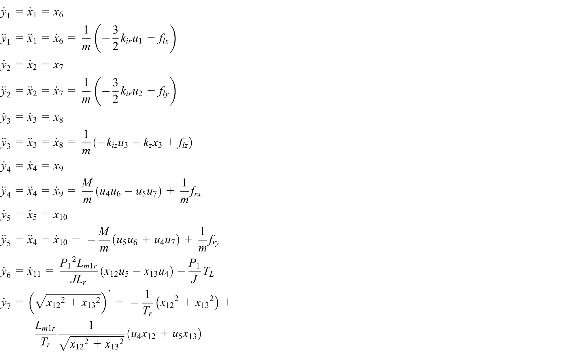
Substituting equations (1), (6), (7), and (9–11) into equation (8), the 13-order state equation of the system can be acquired as follows

{\begin{matrix} {\overset{\cdot}{x}}_{1} = x_{6} \\ {\overset{\cdot}{x}}_{2} = x_{7} \\ {\overset{\cdot}{x}}_{3} = x_{8} \\ {\overset{\cdot}{x}}_{4} = x_{9} \\ {\overset{\cdot}{x}}_{5} = x_{10} \\ {\overset{\cdot}{x}}_{6} = \frac{1}{m} (- \frac{3}{2} k_{ir} u_{1} + f_{lx}) \\ {\overset{\cdot}{x}}_{7} = \frac{1}{m} (- \frac{3}{2} k_{ir} u_{2} + f_{ly}) \\ {\overset{\cdot}{x}}_{8} = \frac{1}{m} (- k_{iz} u_{3} - K_{z} x_{3} + f_{lz}) \\ {\overset{\cdot}{x}}_{9} = \frac{M}{m} (u_{4} u_{6} - u_{5} u_{7}) + \frac{1}{m} f_{rx} \\ {\overset{\cdot}{x}}_{10} = - \frac{M}{m} (u_{5} u_{6} + u_{4} u_{7}) + \frac{1}{m} f_{ry} \\ {\overset{\cdot}{x}}_{11} = \frac{{P_{1}}^{2} L_{m 1 r}}{J L_{r}} (x_{12} u_{5} - x_{13} u_{4}) - \frac{P_{1}}{J} T_{L} \\ {\overset{\cdot}{x}}_{12} = - \frac{1}{T_{r}} x_{12} - x_{11} x_{13} + \frac{L_{m 1 r}}{T_{r}} u_{4} \\ {\overset{\cdot}{x}}_{13} = - \frac{1}{T_{r}} x_{13} + x_{11} x_{12} + \frac{L_{m 1 r}}{T_{r}} u_{5} \end{matrix}

(12)

Reversibility analysis of 5-DOF BIM

To analyze the reversibility of 5-DOF BIM, it needs to keep differentiating the output with respect to time until the input variable exists in the equation. From equation (12), the following equations are obtained

\begin{matrix} {\overset{\cdot}{y}}_{1} = {\overset{\cdot}{x}}_{1} = x_{6} \\ {\overset{\cdot\cdot}{y}}_{1} = {\overset{\cdot\cdot}{x}}_{1} = {\overset{\cdot}{x}}_{6} = \frac{1}{m} (- \frac{3}{2} k_{ir} u_{1} + f_{lx}) \\ {\overset{\cdot}{y}}_{2} = {\overset{\cdot}{x}}_{2} = x_{7} \\ {\overset{\cdot\cdot}{y}}_{2} = {\overset{\cdot\cdot}{x}}_{2} = {\overset{\cdot}{x}}_{7} = \frac{1}{m} (- \frac{3}{2} k_{ir} u_{2} + f_{ly}) \\ {\overset{\cdot}{y}}_{3} = {\overset{\cdot}{x}}_{3} = x_{8} \\ {\overset{\cdot\cdot}{y}}_{3} = {\overset{\cdot\cdot}{x}}_{3} = {\overset{\cdot}{x}}_{8} = \frac{1}{m} (- k_{iz} u_{3} - k_{z} x_{3} + f_{lz}) \\ {\overset{\cdot}{y}}_{4} = {\overset{\cdot}{x}}_{4} = x_{9} \\ {\overset{\cdot\cdot}{y}}_{4} = {\overset{\cdot\cdot}{x}}_{4} = {\overset{\cdot}{x}}_{9} = \frac{M}{m} (u_{4} u_{6} - u_{5} u_{7}) + \frac{1}{m} f_{rx} \\ {\overset{\cdot}{y}}_{5} = {\overset{\cdot}{x}}_{5} = x_{10} \\ {\overset{\cdot\cdot}{y}}_{5} = {\overset{\cdot\cdot}{x}}_{4} = {\overset{\cdot}{x}}_{10} = - \frac{M}{m} (u_{5} u_{6} + u_{4} u_{7}) + \frac{1}{m} f_{ry} \\ {\overset{\cdot}{y}}_{6} = {\overset{\cdot}{x}}_{11} = \frac{{P_{1}}^{2} L_{m 1 r}}{J L_{r}} (x_{12} u_{5} - x_{13} u_{4}) - \frac{P_{1}}{J} T_{L} \\ {\overset{\cdot}{y}}_{7} = {(\sqrt{{x_{12}}^{2} + {x_{13}}^{2}})}^{'} = - \frac{1}{T_{r}} ({x_{12}}^{2} + {x_{13}}^{2}) + \frac{L_{m 1 r}}{T_{r}} \frac{1}{\sqrt{{x_{12}}^{2} + {x_{13}}^{2}}} (u_{4} x_{12} + u_{5} x_{13}) \end{matrix}

The Jacobian matrix is as follows

A (x) = \frac{\partial Y}{\partial u^{T}} [\begin{matrix} \begin{matrix} \frac{\partial {\overset{\cdot\cdot}{y}}_{1}}{\partial u_{1}} & \frac{\partial {\overset{\cdot\cdot}{y}}_{1}}{\partial u_{2}} \\ \frac{\partial {\overset{\cdot\cdot}{y}}_{2}}{\partial u_{1}} & \frac{\partial {\overset{\cdot\cdot}{y}}_{2}}{\partial u_{2}} \end{matrix} & \begin{matrix} \dots & \frac{\partial {\overset{\cdot\cdot}{y}}_{1}}{\partial u_{7}} \\ \dots & \frac{\partial {\overset{\cdot\cdot}{y}}_{2}}{\partial u_{7}} \end{matrix} \\ \begin{matrix} ⋮ & ⋮ \\ \frac{\partial {\overset{\cdot}{y}}_{7}}{\partial u_{1}} & \frac{\partial {\overset{\cdot}{y}}_{7}}{\partial u_{2}} \end{matrix} & \begin{matrix} ⋮ \\ \dots & \frac{\partial {\overset{\cdot}{y}}_{7}}{\partial u_{7}} \end{matrix} \end{matrix}] = [\begin{matrix} - \frac{3 k_{ir}}{2 m} & 0 & 0 & 0 & 0 & 0 & 0 \\ 0 & - \frac{3 k_{ir}}{2 m} & 0 & 0 & 0 & 0 & 0 \\ 0 & 0 & - \frac{k_{iz}}{m} & 0 & 0 & 0 & 0 \\ 0 & 0 & 0 & \frac{M}{m} u_{6} & - \frac{M}{m} u_{7} & \frac{M}{m} u_{4} & - \frac{M}{m} u_{5} \\ 0 & 0 & 0 & - \frac{M}{m} u_{7} & - \frac{M}{m} u_{6} & - \frac{M}{m} u_{5} & - \frac{M}{m} u_{4} \\ 0 & 0 & 0 & - \frac{{P_{1}}^{2} L_{m 1 r}}{J L_{r}} x_{13} & \frac{{P_{1}}^{2} L_{m 1 r}}{J L_{r}} x_{12} & 0 & 0 \\ 0 & 0 & 0 & \frac{L_{m 1 r} x_{12}}{T_{r} \sqrt{{x_{12}}^{2} + {x_{13}}^{2}}} & \frac{L_{m 1 r} x_{13}}{T_{r} \sqrt{{x_{12}}^{2} + {x_{13}}^{2}}} & 0 & 0 \end{matrix}]

(13)

A(x) is nonsingular, rank[ A (x)] = 7; the relative order of the system is α = (α₁, α₂, α₃, α₄, α₅, α₆, α₇) = (2, 2, 2, 2, 2, 1, 1), and $\sum_{j = 1}^{7} α_{j} = 12 < n$ (n is the order of the system). Hence, the system is reversible.

LSSVMI decoupling control of 5-DOF BIM

Identification principle of LSSVM

The identification principle of LSSVM is known that the regress of unknown functions can be realized by selecting a function y( x ) = ω^T φ( x ) + b. x_i ∈ R^m is the weight value vector, b ∈ R is the biasing, and the training samples (x_i, y_i) $(i = 1, 2, \dots, n)$ are mapped from the original space to the high-dimensional feature space by nonlinear mapping function φ(x). The definition of optimization problems of the LSSVM are as follows

{\begin{matrix} min J (ω, ε) = \frac{1}{2} ω^{T} ω + \frac{γ}{2} \sum_{i = 1}^{n} ε_{i}^{2} \\ \begin{matrix} s . t . & y_{i} = ω^{T} φ (x_{i}) + b + ε_{i}, i = 1, 2, \dots n \end{matrix} \end{matrix}

(14)

where γ and ε_i are the relaxation factors of the regularization parameter and the insensitive loss function, respectively. From the Lagrange function of (15), it can be known that the optimization problems of the expression (14) can be solved as follows

L (ω, α, b, ε) = J (ω, ε) - \sum_{i = 1}^{n} a_{i} (y_{i} - ω^{T} φ (x_{i}) - b - ε_{i})

(15)

where a_i is the Lagrange multiplier. According to the optimal conditions of Karush–Kuhn–Tucker, by calculating the partial derivatives of Lagrange function, the answers of optimization problems are shown as follows

[\begin{matrix} 0 & 1 & ⋮ & 1 \\ 1 & K (x_{1}, x_{1}) + \frac{1}{γ} & ⋮ & K (x_{1}, x_{n}) \\ ⋮ & ⋮ & ⋮ \\ 1 & K (x_{n}, x_{1}) & ⋮ & K (x_{n}, x_{n}) + \frac{1}{γ} \end{matrix}] [\begin{matrix} b \\ a_{1} \\ ⋮ \\ a_{n} \end{matrix}] = [\begin{matrix} 0 \\ y_{1} \\ ⋮ \\ y_{n} \end{matrix}]

(16)

where K(x_i, y_j) is the kernel function which satisfies the Mercer condition. This article chooses the radial basis function (RBF) kernel function as the following form

K (x_{i}, x_{j}) = \exp (- \frac{{| x_{i} - x_{j} |}^{2}}{(2 σ^{2})})

(17)

where σ is the width of the kernel. From formula (16), a and b can be obtained, and from formula (15) ω can be obtained. The fitted equation of (x_i, y_i) can be obtained as follows

y (x) = \sum_{i = 1}^{n} a_{i} K (x_{i}, x) + b

(18)

Parameter optimization of LSSVM model

This article uses the PSO algorithm to optimize the kernel width of LSSVM and the regularization parameters. The PSO algorithm is a kind of swarm intelligence optimization technique, which was proposed by Kennedy and Eberhart²⁴ in 1995. Assuming that a group consists of m particles in the D dimension, the ith dimension is expressed as follows

Q_{i} = (u_{i}, v_{i}, p_{i}, p_{g})

(19)

where $u_{i} = [{u_{i}}_{1}, u_{i 2}, \dots, u_{id}]$ and $v_{i} = [{v_{i}}_{1}, v_{i 2}, \dots, v_{id}]$ are the speed and the initial position of Q _i, respectively; $p_{i} = [{p_{i}}_{1}, p_{i 2}, \dots, p_{id}]$ and $p_{i} = [{p_{i}}_{1}, p_{i 2}, \dots, p_{id}]$ are the individual optimal solution and the global optimal solution, respectively; i = 1, 2,…, m; and d = 1, 2,…, D. All the particles in the particle swarm update the velocity and position by equations (20) and (21)

v_{i} (k + 1) = ϖ v_{i} (k) + c_{1} r_{1} (p_{i} (k) - u_{i} (k)) + c_{2} r_{2} (p_{g} (k) - u_{i} (k))

(20)

u_{i} (k + 1) = u_{i} (k) + v_{i} (k)

(21)

where r₁ and r₂ are the random numbers in (0, 1); c₁ and c₂ are the learning factors; and $ϖ$ is the inertia weight.

The sample mean square deviation e_RMSE can be built such as equation (22), which is the performance evaluation index of LSSVM and the objective function of the PSO algorithm

e_{RMSE} = \sqrt{\frac{1}{l} \sum_{i = 1}^{l} {(y_{i} - {\hat{y}}_{i})}^{2}}

(22)

where y_i and ${\hat{y}}_{i}$ are the actual value and the model output value, respectively, i = 1, 2,…, n. When e_RMSE is the minimum, the regularization parameter γ and the kernel width σ are the optimization parameters of LSSVM.

Implementation procedure

Data sample collection. Through the closed-loop PID control of 5-DOF BIM, the training data samples can be obtained. According to the physical operation area of 5-DOF BIM, the given random excitation signals of the speed, flux, and rotor position can be set to collect the response of the real-time system. The training samples of the 5-DOF BIM inverse model are { ${\overset{\cdot\cdot}{x}}_{l}$ , ${\overset{\cdot}{x}}_{l}$ , $x_{l}$ , ${\overset{\cdot\cdot}{y}}_{l}$ , ${\overset{\cdot}{y}}_{l}$ , $y_{l}$ , ${\overset{\cdot\cdot}{z}}_{l}$ , ${\overset{\cdot}{z}}_{l}$ , $z_{l}$ , ${\overset{\cdot\cdot}{x}}_{r}$ , ${\overset{\cdot}{x}}_{r}$ , $x_{r}$ , ${\overset{\cdot\cdot}{y}}_{r}$ , ${\overset{\cdot}{y}}_{r}$ , $y_{r}$ , $\overset{\cdot}{ω}$ , $ω$ , ${\overset{\cdot}{ψ}}_{r}$ , $ψ_{r}$ } and {i_lx, i_ly, i_lz, i_d_1s, i_q_1s, i_d_2s, i_q_2s}. The first- and second-order derivatives of the sample are calculated by five-point derivative algorithm. The sampling period is 0.1 ms and the sampling time is 0.1 s. In total, 1000 groups of sample data are obtained; of which, 400 groups are used as the training sample, and another 400 groups are used as the test sample. They serve to check the identification precision of the 5-DOF BIM inverse model.

LSSVM training. According to the input and output sample data of the LSSVM, the LSSVM is trained, and the 5-DOF BIM inverse model is established. What is more, the PSO algorithm is adopted to optimize the kernel width σ and the regularization parameters γ, so as to make the output value of LSSVM approach to the expectations.

Implementation of LSSVM control. Adding the integrator (S⁻¹) to the trained LSSVM builds the LSSVMI of 5-DOF BIM, which is used as the feed-forward controller in front of the original system. The pseudo linear system consists of LSSVMI and the original system; of which, the input and output are linear decoupling. The pseudo linear system is equivalent to seven decoupling integral linear subsystems. They are five-position second-order integral subsystems, a speed first-order integral subsystem, and a magnetic first-order integral subsystem, respectively. The corresponding transfer functions are G_lx(S) = S⁻², G_ly(S) = S⁻², G_lz(S) = S⁻², G_rx(S) = S⁻², G_ry(S) = S⁻², G_ω(S) = S⁻¹, and G_ψ(S) = S⁻¹. In order to obtain the excellent static and dynamic performances of 5-DOF BIM, the closed-loop controller is designed for pseudo linear subsystems. In this article, the feedback controller is the PID controller with differential limit and integral separation links. Figure 4 shows the LSSVMI decoupling control block diagram of 5-DOF BIM system.

Figure 4.

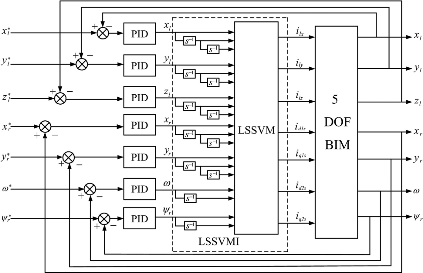
Decoupling control block diagram of the 5-DOF BIM.

Simulation and experimental research

Parameters of prototype

The parameters of 3-DOF RAHMB are shown in Table 1 and the parameters of 2-DOF BIM are shown in Table 2.

Table 1.

Parameters of 3-DOF RAHMB.

Parameters	Radial	Axial
Number of coil turns (r)	280	140
Current stiffness (N/A)	750	750
Displacement stiffness (N/A)	1.0	1.9
Air gap (mm)	0.5	0.5

Table 2.

Parameters of 2-DOF BIM.

Parameters	Torque winding	Suspension winding
Rated power (kW)	1	0.5
Air gap (mm)	2	2
Air gap of auxiliary bearing (mm)	0.5	0.5
Rotor resistance (Ω)	11.48	0.075
Number of coil turns (r)	480	240
Mutual inductance of stator and rotor (H)	0.15856	0.00932
Rotor inductance (H)	0.16778	0.01474
Rotational inertia (kg m²)	0.00769	0.00769
Mutual inductance of two sets of winding (H/m)	78.2	78.2
Rotor time constant (s)	0.0146	0.0146
Rotor weight (kg)	2.85	2.85
Pole pairs	1	2

Simulation analysis

The simulation parameters of PSO are as follows: m = 60, D = 2, c₁ = c₂ = 2, the number of termination iterations is k = 300, and the attenuation of $ϖ$ is from 0.85 to 0.45. The prediction root mean square error (ε_MAXE) and the maximum absolute error (ε_MAXE) are defined as the evaluation indexes to evaluate the prediction performance of LSSVM model in this article. The definition of ε_RMSE is shown in equation (22), and the definition of ε_MAXE is shown as follows

ε_{MAXE} = \max_{i = 1}^{N} | y_{i} - {\hat{y}}_{i} |

(23)

In order to test and verify the effectiveness of the LSSVMI model, the inverse model of 5-DOF BIM is built based on the classic SVM and PSO-LSSVM, respectively. Comparing the ε_RMSE with the ε_MAXE in the 400 groups of the selected test data, the results are shown in Table 3. It shows that the 5-DOF BIM inverse model built by the PSO-LSSVM has better fitting ability and prediction precision.

Table 3.

Comparison of the two kinds of model prediction effect.

	ε _RMSE	ε _MAXE
Classic SVM	0.0932	0.2625
PSO-LSSVM	0.0274	0.0742

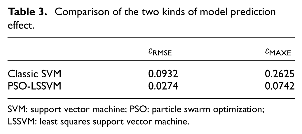
SVM: support vector machine; PSO: particle swarm optimization; LSSVM: least squares support vector machine.

When the rotor of 5-DOF BIM is in the stationary state, x_r = x_l = x and y_r = y_l = y. Figure 5 shows the centroid trajectory of the 5-DOF BIM rotor without load. Assuming the rotor initial displacement value is x = −0.1 mm, y = −0.1 mm. From Figure 5, it can be seen that the rotor centroid trajectory is smooth in the process of rotor floating, and the trajectory can approach to the equilibrium point (0, 0) quickly. It realizes the stable suspension at the equilibrium point. At the same time, the coupling of each DOF is small. The system has good dynamic and static performance.

Figure 5.

Trajectory of the rotor centroid.

In order to verify the decoupling effect of LSSVMI, the system given values change at different time. Figure 6 shows the decoupling effect of speed, flux, and radial displacement in the x-axis of the 5-DOF BIM. Figure 6(a) shows the speed characteristic curve of 5-DOF BIM; Figure 6(b) shows the flux characteristic curve of 5-DOF BIM; Figure 6(c) shows the characteristic curve of radial displacement in the x-axis of 5-DOF BIM. When t = 0.06 s, the flux drops suddenly from 0.8 to 0.4 Wb; when t = 0.1 s, the speed increases suddenly from 3000 to 6000 r/min; when t = 0.12 s, the radial displacement in the x-axis decreases suddenly from 0.18 to 0.12 mm. It can be seen from Figure 6 that the curve response is rapid, the overshoot is small, and one input only affects its own output. Therefore, this system implements the decoupling between speed, flux, and displacement.

Figure 6.

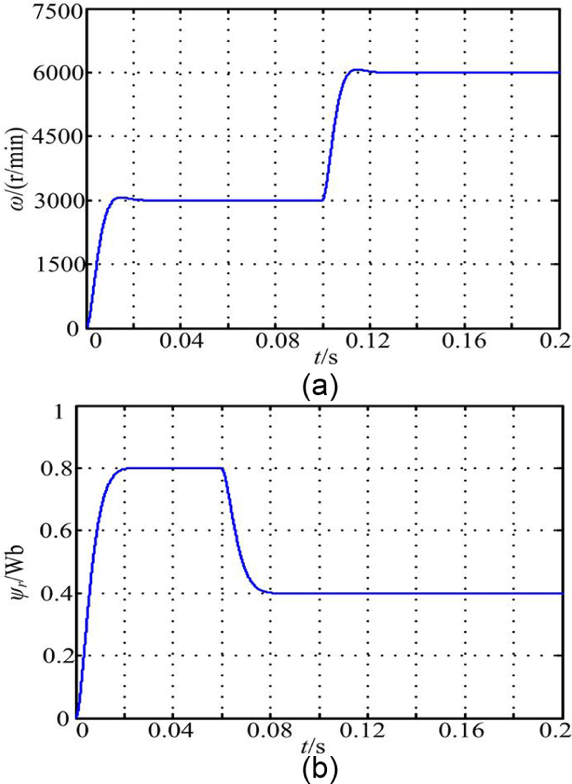
Decoupling effect curve between (a) speed, (b) flux, and (c) x direction displacement.

Figure 7 shows the decoupling effect between x, y, and z direction displacements of 5-DOF BIM. When t = 0.06 s, the displacement in the y direction increases suddenly from 0.05 to 0.15 mm; when t = 0.11 s, the displacement in the x direction changes suddenly from 0.2 to 0.1 mm. The decoupling control result is shown in Figure 7(a). From Figure 7(a), it can be known that one input only affects its own output in the x and y directions; when t = 0.04 s, the displacement in the z direction changes suddenly from 0.175 to 0.125 mm; when t = 0.08 s, the displacement in the x direction changes suddenly from 0.05 to 0.13 mm; the decoupling control result is shown in Figure 7(b). From Figure 7(b), it can be found that one input only affects one output in the x and z directions. Therefore, the system realizes the good decoupling control performance for displacement in the x, y, and z directions.

Figure 7.

Decoupling effect curve between (a) x and y direction displacement and (b) x and z direction displacement.

Experimental analysis

In order to further verify the effectiveness of the LSSVMI decoupling control strategy, the digital control experiment platform is established with a 2-DOF BIM based on the TMS320F28335. In this experiment, the eddy current displacement sensor is used to measure the displacement of x and y directions, and the incremental photoelectric encoder is used to measure the speed. In addition, the commonly current speed observer is used to observe the rotor flux. The LSSVMI control algorithm is realized by the TMS320F28335. The experimental results are shown in Figure 8.

Figure 8.

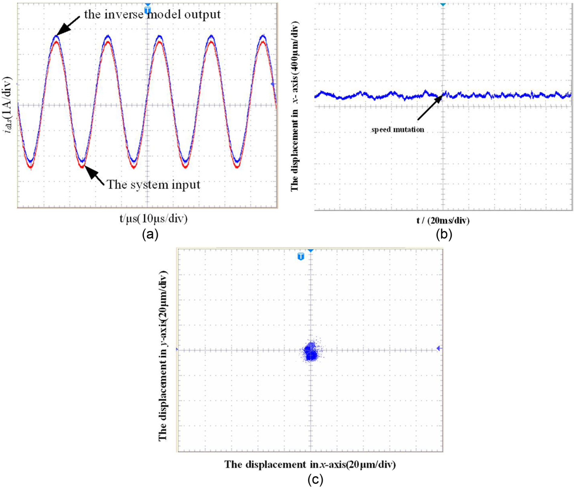
Experimental results: (a) the system input and LSSVMI model output, (b) x direction displacement under speed mutation, and (c) the rotor centroid trajectory.

Figure 8(a) shows the input current i_d_1s of system and the corresponding output model current based on LSSVMI. It can be seen from Figure 8(a) that the LSSVMI model has good regress for the input of system, which means that the LSSVMI model optimized by the PSO optimization algorithm has higher fitting and forecasting precision. Figure 8(b) shows the waveform of the displacement in the x direction when the speed suddenly increases from 1200 to 2400 r/min. When the motor speed increases suddenly, the radial vibration amplitude of rotor at the center equilibrium position keeps steadiness, and the peak–peak value is <40 µm. It implements the dynamic decoupling between the speed and the radial displacement. Figure 8(c) shows the waveform of rotor centroid trajectory when the speed is 2400 r/min. The rotor centroid trajectory distributes at the intersection point of x- and y-axes (around the center of equilibrium position). The maximum values of the centroid displacement in the x- and y-axes are 16 and 20 µm, respectively. The motor is in a stable suspension state. From Figure 8(a)–(c), it can be known that using the new decoupling control strategy, the rotor realizes the steady and dynamic suspended operations, and the performance of decoupling control is good.

Conclusion

In order to achieve the high-performance control of 5-DOF BIM, the LSSVM inverse control strategy based on the PSO optimization algorithm is proposed to research the nonlinear decoupling control, and the conclusions are as follows:

The nonlinear decoupling control of 5-DOF BIM system is realized successfully by LSSVMI decoupling control strategy, and the simulation results illustrate that the system has excellent dynamic and static performances, and it has strong robustness to the model errors.

In order to identify the inverse system model better by LSSVM, the PSO algorithm is applied to optimize the LSSVM parameters. The simulation and preliminary experiments show that the inverse model has a higher fitting and predicted precision.

Limited by the experiment conditions, the experiment research is carried out on the digital control experiment platform with a 2-DOF BIM. It realizes a dynamic decoupling control between the speed and displacement and verifies the effectiveness of the proposed control strategy, which also, creates solid foundation for the next step to achieve the experiment research based on the LSSVMI 5-DOF BIM.

Footnotes

Academic Editor: José Tenreiro Machado

Declaration of conflicting interests

The author(s) declared no potential conflicts of interest with respect to the research, authorship, and/or publication of this article.

Funding

The author(s) disclosed receipt of the following financial support for the research, authorship, and/or publication of this article: This work was supported by the National Natural Science Foundation of China under projects 51475214, 61104016, and 51305170; the China Postdoctoral Science Foundation–funded project under project 2015T80508; the Natural Science Foundation of Jiangsu Province of China under projects BK20130515, BK20141301, and BK20150524; the Professional Research Foundation for Advanced Talents of Jiangsu University under projects BK20150524 and 14JDG076; Six Categories Talent Peak of Jiangsu Province under projects ZBZZ-017 and 2015-XNYQC-003; and the Priority Academic Program Development of Jiangsu Higher Education Institutions (PAPD).

References

Sun

Chen

Yang

Overview of bearingless induction motors. Math Probl Eng 2014; 2014: 570161.

Yang

Dong

Gao

. Rotor mass eccentricity vibration compensation control in bearingless induction motor. Adv Mech Eng 2015; 7: 168428.

Fang

Zheng

Han

Attitude sensing and dynamic decoupling based on active magnetic bearing of MSDGCMG. IEEE T Instrum Meas 2012; 61: 338–348.

Sun

Chen

Jiang

. High-performance control for a bearingless permanent-magnet synchronous motor using neural network inverse scheme plus internal model controllers. IEEE T Ind Electron 2016; 63: 3479–3488.

Chiba

Santisteban

JA.

A PWM harmonics elimination method in simultaneous estimation of magnetic field and displacements in bearingless induction motors. IEEE T Ind Appl 2012; 48: 124–130.

Sun

Chen

Yang

Overview of bearingless permanent-magnet synchronous motors. IEEE T Ind Electron 2013; 60: 5528–5538.

Lapotre

Takorabet

Meibody-Tabar

. New model of radial force determination in bearingless motor. IEEE T Magn 2015; 51: 1–4.

Sun

Chen

Yang

. Analysis of inductance characteristics for a bearingless permanent magnet synchronous motor. Electr Eng 2013; 95: 277–286.

Yang

Wan

Sun

. Sliding mode variable structure control of a bearingless induction motor based on a novel reaching law. Energies 2016; 9: 452.

10.

Sun

Xue

Chen

. Radial position control of a magnetically suspended rotor system in a direct-driven spindle using inverse system scheme. T I Meas Control 2016; 38: 1073–1086.

11.

Fang

Sun

Liu

. A novel 3-DOF axial hybrid magnetic bearing. IEEE T Magn 2010; 46: 4034–4045.

12.

Sun

Zhu

Artificial neural networks inverse control of 5 degrees of freedom bearingless induction motor. Int J Model Ident Contr 2012; 15: 156–163.

13.

. Inverse system decoupling control strategy of BLIM based on stator flux orientation. Int J Appl Electrom 2015; 48: 469–480.

14.

Sun

Zhu

Yang

Speed-sensorless operation of bearingless induction motor based on left-inverse system. Control Decis 2012; 27: 1256–1260.

15.

Zhu

Zhou

YH.

Mathematical model and control of magnetic bearings based on α-th order inverse system theory. Electr Mach Control 2009; 13: 406–501 (in Chinese with English abstract).

16.

Sun

Chen

Yang

. Speed-sensorless vector control of a bearingless induction motor with artificial neural network inverse speed observer. IEEE/ASME T Mech 2013; 18: 1357–1366.

17.

Wang

Liu

Nonlinear internal model control for bearingless induction motor based on neural network inversion. Acta Automat Sin 2013; 39: 433–439 (in Chinese with English abstract).

18.

Suykens

JAK

Vandewalle

. Recurrent least squares support vector machines. IEEE T Circuits: I 2000; 47: 1109–1114.

19.

Sun

Zhu

Yang

Application of LSSVM inverse in a variable frequency induction motor drive system. T I Meas Control 2013; 35: 247–254.

20.

Jin

Zhou

. Research and application of the reversed modeling method and partial least-square regression modeling for the complex thermal system. Proc Chin Soc Electr Eng 2009; 29: 25–29 (in Chinese with English abstract).

21.

Zhu

Cao

. Decoupling control of 5-degree of freedom bearingless synchronous reluctance motor based on least square support vector machine inverse system. Proc Chin Soc Electr Eng 2013; 33: 99–108 (in Chinese with English abstract).

22.

Sun

Zhu

Yang

Nonlinear modeling of flux linkage for a bearingless permanent magnet synchronous motor with modified particle swarm optimization and least squares support vector machines. J Comput Theor Nanos 2013; 10: 416–422.

23.

Chao

Lijun

An optimum allocation method of voltage sag monitoring nodes based on particle swarm optimization algorithm. Trans China Electrotech Soc 2014; 29: 181–187 (in Chinese with English abstract).

24.

Kennedy

Eberhart

RC.

Particle swarm optimization. In: Proceedings of the international conference on neural networks, Perth, WA, Australia, 27 November–1 December 1995, pp.1942–1948. New York: IEEE.

25.

Sun

Chen

. Nonlinear flux linkage modeling of a bearingless permanent magnet synchronous motor based on AW-LSSVM regression algorithm. Int J Appl Electrom 2016; 51: 151–159.

26.

Zhang

Sun

Tang

. Service composition based on discrete particle swarm optimization in military organization cloud cooperation. J Syst Eng Electron 2016; 27: 590–601.

Decoupling control of a 5-degree-of-freedom bearingless induction motor based on least squares support vector machine inverse

Abstract

Keywords

Introduction

Basic structure and mathematics model of 5-DOF BIM

Mathematical model of 3-DOF RAHMB radial–axial suspension force

Mathematical model of 2-DOF BIM

Mathematical model of 5-DOF BIM

Reversibility analysis of 5-DOF BIM

LSSVMI decoupling control of 5-DOF BIM

Identification principle of LSSVM

Parameter optimization of LSSVM model

Implementation procedure

Simulation and experimental research

Parameters of prototype

Simulation analysis

Experimental analysis

Conclusion

Footnotes

Declaration of conflicting interests

Funding

References