Sage Journals: Discover world-class research

Abstract

For the inverse proposition design of a three-dimensional centrifugal impeller using the streamline curvature method, the cubic spline curve fitting method is extensively used to solve the velocity gradient equation. Given the deficiency in stability with the cubic spline curve fitting method, a new finite difference method is proposed to solve the velocity gradient equation on the S2m stream surface. In the finite difference scheme, the relative velocity derivative along the streamline direction is decomposed into two terms. One term uses forward difference, and the other uses backward difference. The difference schemes of all other parameter derivatives in the velocity gradient equation adopt forward difference. The method can guarantee the matrix main diagonal elements of the dominant, indicating stable convergence in solving the velocity field. Robustness analysis is performed for both methods, and the new finite difference method shows excellent superiority in stability. Finally, the finite difference method is applied to redesign the Krain impeller. Through computational fluid dynamics, the efficiency of the redesigned impeller at the design operating point is increased by approximately 0.3% and the pressure ratio by approximately 5%. These results show that the difference method is feasible to solve the S2m stream surface velocity gradient equation.

Keywords

Finite difference method streamline curvature S2m stream surface velocity gradient equation inverse proposition centrifugal compressor design

Introduction

The streamline curvature method plays an important role in the preliminary design phase of radial^1–4 and axial turbomachinery applications⁵ because of its simple and compact equations, definite physical meanings, and straightforward solving algorithm. In the method, the velocity profile on the stream surface is specified by solving the S2m stream surface velocity gradient equation. Then, the blade profile can be shaped based on the given variations in design parameters.

Most through flow codes use the streamline curvature method and derive from those of Hamrick et al.,⁶ Smith,⁷ and Novak,⁸ based on the general theory of Wu.⁹ The cubic spline function and quasi-orthogonal grids were applied to the streamline curvature method to enhance its accuracy and efficiency in calculation.¹⁰ With the method, the blade shape is generated by specifying the distributions of relative velocity on both pressure and suction surfaces along the streamline direction.¹¹ Considering that secondary flow and turbulent diffusion play important roles in the mixing process,^12,13 Casey and Robinson¹⁴ proposed a new model applied to the streamline curvature method for spanwise mixing of angular momentum, total enthalpy, and entropy across the meridional streamtubes.

However, the streamline curvature method exhibits deficiency in stability.^15–17 First, an appropriate initialization is necessary because the convergence of calculation is susceptible to the initial values. Second, because of the requirement of grid node adjustment during the iteration, guaranteeing the smoothness of the streamlines is difficult. In practice, the cubic spline curve fitting method is extensively used to solve the inverse proposition of streamline curvature method.^16,18 In addition to simplicity and practicability, satisfactory accuracy can be obtained even if coarse grids are used. However, divergent solutions can appear in certain cases. The analysis for the stability and convergence of the algorithm can be rather difficult. Therefore, the stability analysis of the streamline curvature method still deserves investigation.

For the inverse proposition design of a full three-dimensional (3D) centrifugal impeller with streamline curvature method, this article proposes a new finite difference method to solve the velocity gradient equation. A simplified theoretical derivation and robustness analysis of the proposed method then follows. Finally, the method is applied to redesign the Krain impeller. Through a computational fluid dynamics (CFD) analysis, both the performance and flow field are compared to verify the feasibility of the method.

The velocity gradient equation

For the design of a full (3D) centrifugal impeller, the velocity gradient equation on the S2m stream surface is solved. The velocity gradient equation can be derived from a combination of the first law of thermodynamics, the Euler equation of turbomachinery, and the inviscid momentum equation in a cylindrical coordinate system for the flow on the mean stream surface, such as the following form

\frac{d W_{m}}{dq} = A W_{M} + B + \frac{C}{W_{M}}

(1)

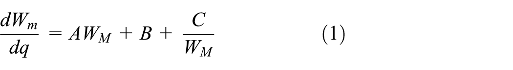
where

\begin{matrix} A = \frac{\cos (α - ψ)}{r_{c}} \\ B = \frac{d (r C_{θ})}{dm} \frac{d θ}{dq} - \frac{d (r C_{θ})}{dq} \frac{d θ}{dm} + \frac{d W_{m}}{dm} \sin (α - ψ) \\ C = - T \frac{d S_{e}}{dq} + \frac{{dh}_{in}^{*}}{dq} - ω \frac{d {(r C_{θ})}_{in}}{dq} \\ θ = \int_{m_{out}}^{m} \frac{r C_{θ} - ω r^{2}}{r^{2} W_{m}} dm + θ_{out} \end{matrix}

The velocity gradient equation, equation (1), is derived from the inviscid flow equation. Viscidity shows little influence on the solution to the flow field in the case of no boundary-layer separation of the main flow in the impeller. The effect of the boundary layer on the flow field can be considered by assigning the efficiency profile along the meridional streamlines. The influences of viscidity and boundary layer are both considered because the entropy along the gradient direction of the quasi-orthogonal curve in equation (1) depends on the given efficiency profile.

The cubic spline scheme to solve the velocity gradient equation

When applying the cubic spline scheme to solve the velocity gradient equation, the main procedure is to calculate the variables like $r_{c}$ , $d (r C_{θ}) / dm$ , $d θ / dq$ , $d (r C_{θ}) / dq$ , $d θ / dm$ , and $d S_{ε} / dq$ with the cubic spline curve fitting method. $d W_{m} / dq$ could be derived if the variables above were substituted into equation (1). Then, the distribution of velocity field can be obtained with the numerical integration. During the process of solving the velocity field, the magnitude of the velocity at hub side should be adjusted to satisfy mass flow conservation for each quasi-orthogonal curve. On the foundation of mass flow conservation for each quasi-orthogonal curve, the position of each inner streamline was also adjusted for the requirement of mass flow conservation. The approach of adjustment of streamlines can be written as

r_{i, j}^{n + 1} = RF \cdot (\frac{j - 1}{M - 1} \frac{G^{*}}{G_{i, j}} - 1) r_{i, j}^{n} + r_{i, j}^{n}

(2)

where RF is the relaxation factor, M is the number of streamlines, G^* is the design mass flow, G_i,j is the calculated mass flow at the node (i,j), $r_{i, j}^{n}$ is the node coordinate at nth iteration, and $r_{i, j}^{n + 1}$ is the node coordinate at (n + 1)th iteration.

The error in streamlines is defined as

ε_{D} = \frac{| r_{i, j}^{n + 1} - r_{i, j}^{n} |}{r_{i, j}^{n}}

(3)

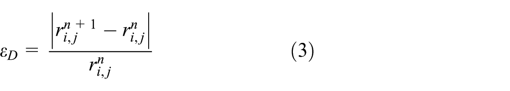
Figure 1 shows the flowchart of streamline curvature inverse proposition with the cubic spline method.

Figure 1.

Flowchart of streamline curvature inverse proposition with the cubic spline method.

Finite difference scheme to the velocity gradient equation

The full 3D blade can be designed by solving the velocity gradient equation, which is a binary differential equation of θ and W_m. The discrete schemes of different terms in the equation are as follows:

1. $d W_{m} / dq$

This term adopts forward difference and is given by

\frac{d W_{m}}{dq} = \frac{{(W_{m})}_{i, j + 1} - {(W_{m})}_{i, j}}{q_{i, j + 1} - q_{i, j}}

(4)

2. $d (r C_{θ}) / dm$ , $d θ / dq$ , $d (r C_{θ}) / dq$ , $d θ / dm$ , and $d S_{ε} / dq$

During the inner iteration for $W_{m}$ , discretizations of these terms have no influence on the convergence of the iterative algorithm, except for an update of θ value. Therefore, forward scheme is adopted to discretize all these terms.

3. $d W_{m} / dm$

The factor of the term $d W_{m} / dm$ is $\sin (α - ψ)$ . The values of α and ψ range from 0 to π/2 along the meridional streamlines of a centrifugal impeller; thus, we obtain $α - ψ$ , which lies between −π/2 and π/2. In other words, the factor can be negative or positive. If we simply adopt a forward difference or backward difference scheme, then the forward difference scheme is taken as an example. The difference scheme of this term can be expressed as

\frac{d W_{m}}{dm} \sin (α - ψ) = \frac{{(W_{m})}_{i + 1, j} - {(W_{m})}_{i, j}}{m_{i + 1, j} - m_{i, j}} \sin (α - ψ)

(5)

On the basis of the velocity gradient equation, equation (1), the difference scheme is as follows

\frac{{(W_{m})}_{i, j + 1} - {(W_{m})}_{i, j}}{q_{i, j + 1} - q_{i, j}} = A (W_{m})_{i, j} + \frac{{(W_{m})}_{i + 1, j} - {(W_{m})}_{i, j}}{m_{i + 1, j} - m_{i, j}} \sin (α - ψ) + k

(6)

where

k = \frac{d (r C_{θ})}{dm} \frac{d θ}{dq} - \frac{d (r C_{θ})}{dq} \frac{d θ}{dm} + \frac{C}{W_{m}}

Then, equation (6) can be reduced to

a_{i, j} (W_{m})_{i, j} = a_{i + 1, j} (W_{m})_{i + 1, j} + a_{i, j + 1} (W_{m})_{i, j + 1} + k

(7)

where

\begin{matrix} a_{i + 1, j} = - \frac{\sin (α - ψ)}{m_{i + 1, j} - m_{i, j}} \\ a_{i, j + 1} = \frac{1}{q_{i, j + 1} - q_{i, j}} \\ a_{i, j} = - a_{i + 1, j} - a_{i, j + 1} - A \end{matrix}

Considering that $α - ψ$ ranges from −π/2 to π/2, the factor A is absolutely non-negative according to the definition. When $α - ψ < 0$ , the matrix main diagonal elements of the dominant can be ensured. That is

| (\frac{\sin (α - ψ)}{m_{i + 1, j} - m_{i, j}} - \frac{1}{q_{i, j + 1} - q_{i, j}} - A) | > | \frac{1}{q_{i, j + 1} - q_{i, j}} | + \frac{\sin (α - ψ)}{m_{i + 1, j} - m_{i, j}}

However, guaranteeing the matrix main diagonal elements of the dominant is difficult when $α - ψ > 0$ because the stability of the difference scheme depends on the value of factor A. Therefore, the stability in solving the velocity field can be poor if a forward difference or backward difference scheme is simply adopted.

To improve the stability and convergence in solving the velocity gradient equation, this term is decomposed into two parts

\frac{d W_{m}}{dm} \sin (α - ψ) = \frac{d W_{m}}{dm} (\sin α \cos ψ - \cos α \sin ψ)

(8)

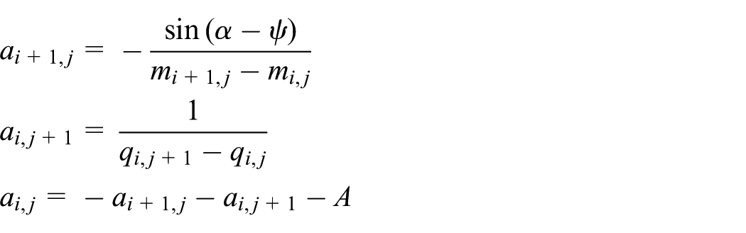
The two terms at the right side of equation (8) can be expressed as follows. One uses forward difference, and the other uses backward difference. The new difference scheme is written as

\frac{d W_{m}}{dm} \sin (α - ψ) = \frac{{(W_{m})}_{i, j} - {(W_{m})}_{i - 1, j}}{m_{i, j} - m_{i - 1, j}} \sin α \cos ψ - \frac{{(W_{m})}_{i + 1, j} - {(W_{m})}_{i, j}}{m_{i + 1, j} - m_{i, j}} \cos α \sin ψ

(9)

Similarly, substituting the new scheme into equation (1) derives the following

a_{i, j} (W_{m})_{i, j} = a_{i - 1, j} (W_{m})_{i - 1, j} + a_{i + 1, j} (W_{m})_{i + 1, j} + a_{i, j + 1} (W_{m})_{i, j + 1} + k

(10)

where

\begin{matrix} a_{i - 1, j} = - \sin α \cos ψ / (m_{i, j} - m_{i - 1, j}) \\ a_{i + 1, j} = - \cos α \sin ψ / (m_{i + 1, j} - m_{i, j}) \\ a_{i, j + 1} = - 1 / (q_{i, j + 1} - q_{i, j}) \\ a_{i, j} = a_{i - 1, j} + a_{i + 1, j} + a_{i, j + 1} - A \end{matrix}

In this way, the matrix main diagonal elements of the dominant can be ensured because of the non-negative factor A, which can be expressed as follows

| \frac{1}{q_{i, j + 1} - q_{i, j}} + \frac{\sin α \cos ψ}{m_{i, j} - m_{i - 1, j}} + \frac{\cos α \sin ψ}{m_{i + 1, j} - m_{i, j}} + A | > | \frac{1}{q_{i, j + 1} - q_{i, j}} | + | \frac{\sin α \cos ψ}{m_{i, j} - m_{i - 1, j}} | + | \frac{\cos α \sin ψ}{m_{i + 1, j} - m_{i, j}} |

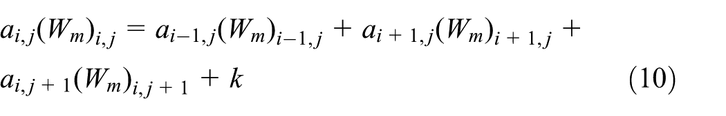
In consideration of the coefficient matrix main diagonal elements of the dominant in solving the velocity gradient equation with the proposed difference method, the Jacobi iteration method can be used directly. In the iteration, the theoretical value of $W_{m}$ (defined as $W_{m}^{*}$ ) satisfies the following

a_{i, j} (W_{m}^{*})_{i, j}^{n + 1} = a_{i - 1, j} (W_{m}^{*})_{i - 1, j}^{n} + a_{i + 1, j} (W_{m}^{*})_{i + 1, j}^{n} + a_{i, j + 1} (W_{m}^{*})_{i, j + 1}^{n} + k

(11)

Subtracting equation (11) from equation (10) and letting $(W_{m})_{i, j} - (W_{m}^{*})_{i, j} = e_{i, j}$ , we have

a_{i, j} e_{i, j}^{n + 1} = a_{i - 1, j} e_{i - 1, j}^{n} + a_{i + 1, j} e_{i + 1, j}^{n} + a_{i, j + 1} e_{i, j + 1}^{n} + \frac{C}{(W_{m})_{i, j}^{n}} - \frac{C}{(W_{m}^{*})_{i, j}^{n}}

(12)

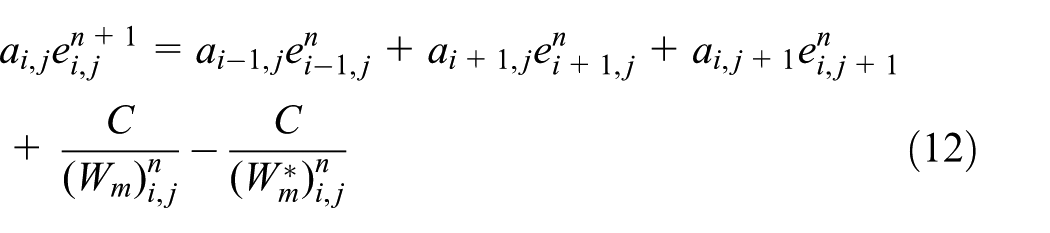
Suppose that the factor C can be neglected for a smaller effect on convergence, equation (12) can then be reduced to

\begin{array}{l} | e_{i, j}^{n + 1} | = | (a_{i - 1, j} e_{i - 1, j}^{n} + a_{i + 1, j} e_{i + 1, j}^{n} + a_{i, j + 1} e_{i, j + 1}^{n}) / a_{i, j} | \\ \leq | (a_{i - 1, j} + a_{i + 1, j} + a_{i, j + 1}) / a_{i, j} | \max_{i = 1, Q} | e_{i, j}^{n} | \leq \max_{i = 1, Q} | e_{i, j}^{n} | \end{array}

In summary, although the simplified derivation is not rigorous, the matrix main diagonal elements of the dominant can be ensured with the proposed finite difference scheme. The proposed scheme shows an obvious advantage compared with simply adopting a forward difference or backward difference scheme. Therefore, on condition that the effect of factor C is neglected, the numerical algorithm can be demonstrated stably convergent. Further robustness analysis is described in the following part.

The flowchart of the streamline curvature inverse proposition program with the finite difference method is presented in Figure 2. Compared to the cubic spline method, two major improvements were made in the algorithm of the finite difference method. One is the improvement of the algorithmic flow. In the finite difference method, three loops were applied to guarantee the convergence of the velocity field, θ-coordinate of the blade and streamlines. The other is the improvement of solving scheme. The finite difference scheme is adopted in place of the cubic spline fitting method. The approach of adjustment of streamlines applying the finite difference method is the same as that of cubic spline fitting method.

Figure 2.

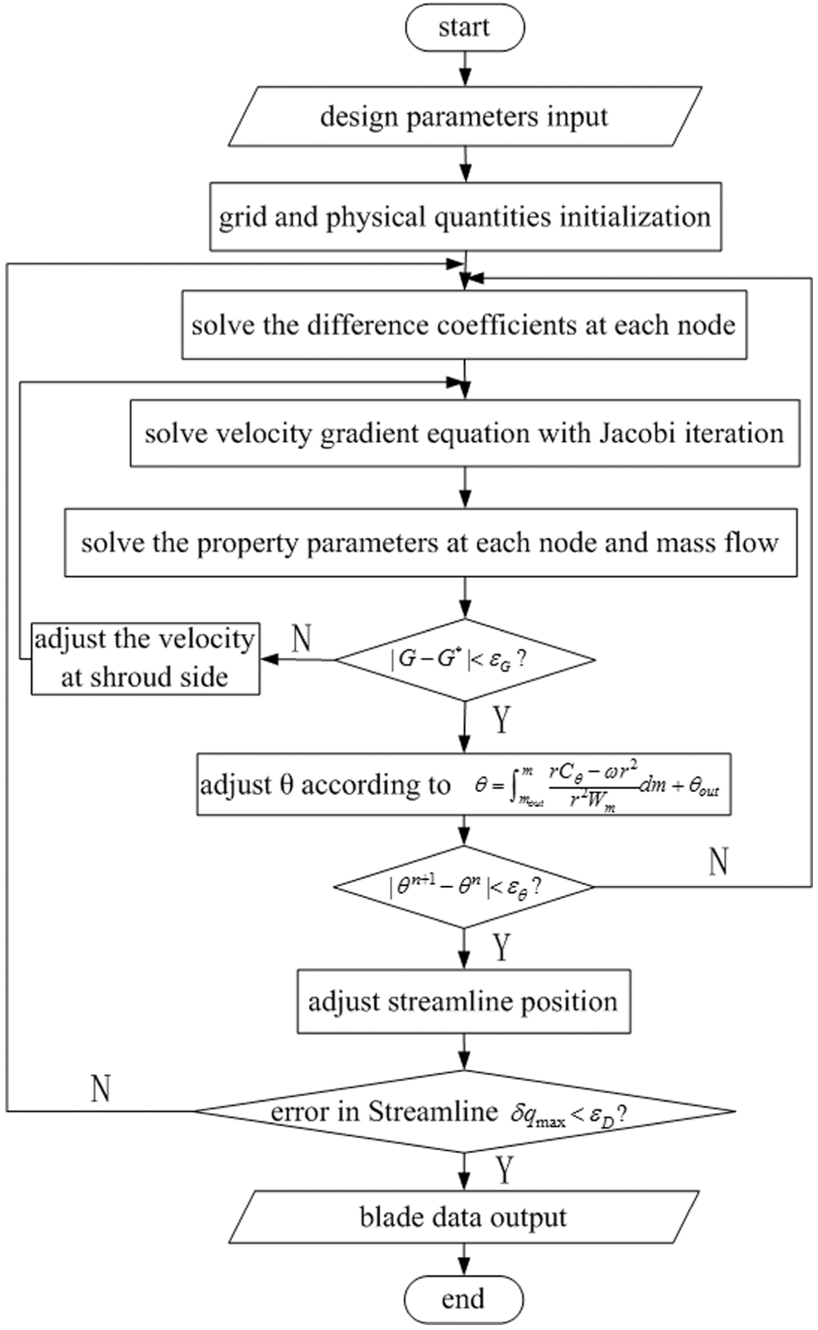
Flowchart of streamline curvature inverse proposition with the finite difference method.

Robustness analysis

Robustness analysis is performed to examine the convergence of the new proposed finite difference method in comparison with the cubic spline method. Figure 3 shows the streamline relative residual curves of both numerical methods with a change in the relaxation factor. It can be seen from Figure 3 that with the same relaxation factor of 0.006, the cubic spline method (solid curve) and the finite difference method (dashed curve) display almost coincident residual history except for the better initial iterations for the finite difference method. However, with a slight increase in the relaxation factor, convergent solutions cannot be obtained in the case of applying the cubic spline method. As for the finite difference method, even if the relaxation factor increases to 0.055, the relative residual curve exhibits great convergence, as shown by the dash dot curve in Figure 3. The numerical program that takes a lower relaxation factor intends to ensure stability at the cost of a longer iteration time. By contrast, if convergent solutions with a much higher relaxation factor can be obtained, apart from the economy in calculation time, it will also be a powerful demonstration for the robustness of the numerical method. When the relaxation factor increases from 0.006 to 0.05, the time consumed for calculation successfully reduces by half from 45.35 to 22.5 s.

Figure 3.

Streamline relative residual curves of the cubic spline method and the finite difference method with the relaxation factors of 0.006 and 0.055.

Figure 4(a)–(c) displays the converged velocity field of both methods and the CFD result for Krain impeller at meridional plane. As shown in Figure 4, there exist some differences in the converged velocity field between the finite difference method and the cubic spline fitting method. When compared with CFD result of Krain impeller, the velocity field of the finite difference method is closer than that of the cubit spline fitting method, especially in the region of high relative velocity gradient. It must be admitted that the results of the finite difference method is imprecise. However, as a relative simple design method, the finite difference method shows acceptable computational accuracy.

Figure 4.

The converged velocity field of both methods and the CFD result for Krain impeller at meridional plane: (a) converged velocity field of the finite difference method, (b) converged velocity field of the cubic spline fitting method, and (c) CFD velocity field of the Krain impeller.

The streamline relative residual curve of the cubic spline method with the relaxation factor of 0.007 is shown in Figure 5. The figure displays a divergent residual curve after several iterations. The velocity distribution for the cubic spline method with the relaxation factors of 0.007 in Figure 6 seems to provide some information for the reason of divergence. As mentioned above, the magnitude of the velocity at hub side should be adjusted to satisfy the mass flow conservation for each quasi-orthogonal curve. However, even if the velocity at hub side upstream of impeller inlet decreases to zero, as shown in Figure 6, the mass flow conservation can be no longer satisfied. This may be one of the reasons leading to calculation divergence. In addition, another instability factor when adopting the cubic spline method can be observed from Figure 6. Instead of a continuous distribution, the velocity at the impeller inlet presents a significant wave fluctuation with peak and valley values appearing alternately. The fluctuation in the velocity can also be observed with the relaxation factors of 0.006 during the initial period of iterations. But the phenomenon disappears gradually with the reduction of error in streamlines. On the contrary, the velocity fluctuation phenomenon does not occur in the case of the finite difference method even if the first iteration is conducted to adjust the streamlines. It is difficult to analyze the reason responsible for the phenomenon when the cubic spline fitting method was applied. It is because both the cubic spline fitting and numerical integration are non-linear computation processes which are used in calculating the velocity distribution. In this article, the reason for this kind of instability is ascribed to the inherent chaos of the algorithm flow itself. It can be seen from Figure 1 that the velocity field is obtained by solving the equation of continuity with numerical integration method. During the process of iterations, calculation for θ-coordinate of the blade is not involved. However, equation (1) indicates that the distribution of the velocity is related to the θ-coordinate of the blade. Therefore, the iteration method in which the θ-coordinate and the velocity are not adjusted simultaneously does not always satisfy the velocity gradient equation. Indeed, the matching of the θ-coordinate and the velocity field is conducted in the outer loop. This explains why the phenomenon of fluctuation in the velocity disappears gradually with the reduction of streamline error. It can be concluded that it is possible to improve the stability of the algorithm by adjusting the calculation flow in Figure 1. For example, an inner loop can be added to judge the matching status of the θ-coordinate and the velocity field. Even so, it is difficult to analyze the matching status because the algorithm involves the convergence analysis of the non-linear calculation. This is why the finite difference method is superior to the cubic spline fitting method in solving the velocity gradient equation.

Figure 5.

The streamline relative residual curve of the cubic spline method with the relaxation factors of 0.007.

Figure 6.

The velocity distribution for the cubic spline method with the relaxation factors of 0.007.

In conclusion, the proposed finite difference method shows better robustness and superiority in the convergence analysis compared with the cubic spline method.

Case design

To validate the proposed difference scheme in this study, this method was applied to redesign the Krain impeller.^19,20 A summary of the design parameters of this impeller is shown in Table 1. The geometrical profile of the Krain impeller is obtained from published literature.²¹ The calculation grids for the redesigned impeller are composed of 10 streamlines and 50 quasi-orthogonal lines. Each quasi-orthogonal line is created by two corresponding points equally divided on the shroud and hub sides. Figure 7 shows the initial grids for redesigned impeller calculation.

Table 1.

Design parameters of the Krain impeller.

Parameters	Value	Unit
Mass flow	4.0	kg s⁻¹
Revolution	22,363	r min⁻¹
Blade number	24
Inlet total pressure	101.325	kPa
Inlet total temperature	15.0	°C
Pressure ratio	4.7

Figure 7.

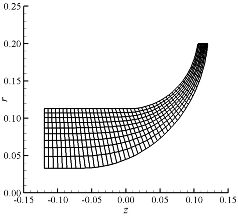
Initial calculation grids for the redesigned impeller.

The circulation profiles along the meridional streamline for blade design at the shroud and hub sides are presented in Figure 8. The circulation profiles are interpolated by a cubic polynomial fitting at both sides for the advantage of the second-order continual derivative property. The expression can be written as

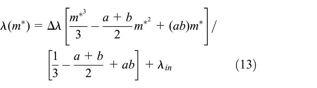
λ (m^{*}) = Δ λ [\frac{m^{*^{3}}}{3} - \frac{a + b}{2} m^{*^{2}} + (ab) m^{*}] / [\frac{1}{3} - \frac{a + b}{2} + ab] + λ_{in}

(13)

where λ is the circulation represented as $r C_{θ}$ , and $Δ λ$ is the circulation variation between impeller inlet and outlet related to Euler work with the design values of 84.0 at the hub side and 82.0 at the shroud side. $m^{*}$ is the normalized distance along meridional streamline, $λ_{in}$ is the circulation at impeller inlet with a given value of 0 at both sides, and a and b are assigned the values 0 and 1.3, respectively, representing the extreme points of the circulation profile.

Figure 8.

Circulation profile.

The abscissa $m^{*} = 0$ in Figure 8 corresponds to the impeller inlet that imposed $d W_{m} / dm = 0$ as the impeller inlet boundary condition. The meridional velocity profile of the redesigned impeller is predicted according to the design parameters, as illustrated in Figure 9. Figure 10 depicts the schematic of the original Krain impeller and the redesigned impeller. The redesigned impeller is a full 3D centrifugal impeller. A major improvement can be recognized from the curved leading edge of the redesigned impeller in comparison to the original straight one.

Figure 9.

Predicted meridional velocity profile of the Krain impeller.

Figure 10.

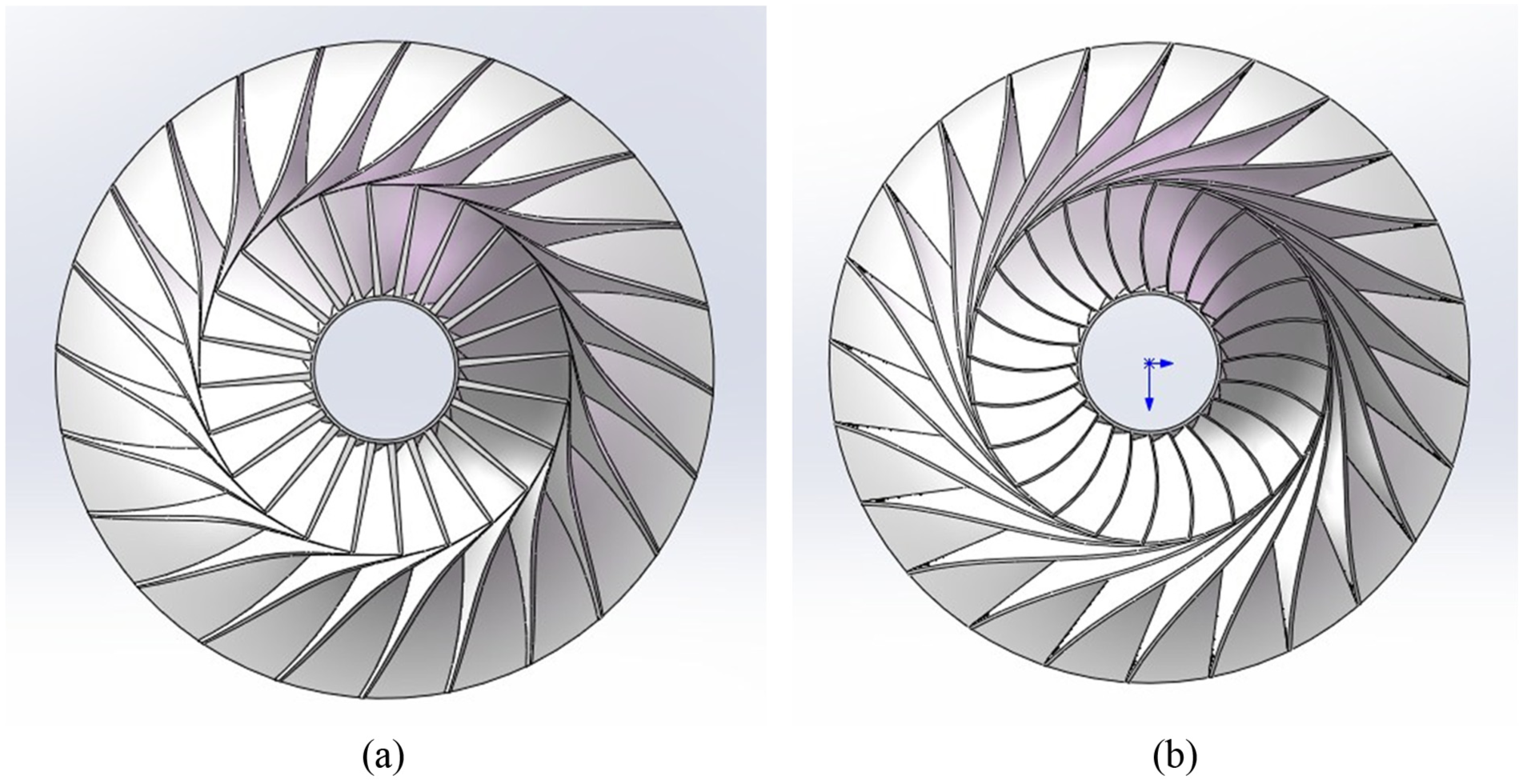
Schematic of both impellers: (a) Krain impeller and (b) redesigned impeller.

Numerical analysis

For the purpose of performance comparison and flow field analysis, both impellers are simulated using commercial software CFX together with a k-ε model. The single impeller passage is selected and a periodic boundary condition is applied at the middle of the blade passage. Total pressure is imposed as the inlet boundary, and the exit boundary condition is given with the mass flow rate. All solid walls are assumed adiabatic. The calculation model of the single impeller passage is shown in Figure 11.

Figure 11.

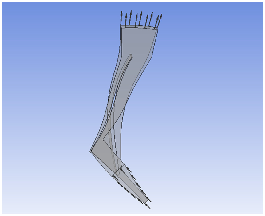
Calculation model of the single impeller passage.

Figures 12 and 13 display the impeller performance curves of both impellers. The experiment data of the Krain impeller in Krain¹⁹ are plotted in Figure 8. Although the experiment measurements of the redesigned impeller are absent because of the limitation of test condition, the discrepancy in efficiency of the simulation results is less than 1% compared with the experimental results of the Krain impeller. The CFD results agree well with the experimental data overall, verifying the reliability of the simulation to some extent. The simulated performance of both impellers shows little difference. The efficiency of the redesigned impeller at the design operating point is increased by approximately 0.3%, while the pressure ratio is increased by approximately 5%.

Figure 12.

Impeller efficiency curve.

Figure 13.

Impeller pressure ratio curve.

For the analysis of the detailed flow field of both impellers, the secondary flow of the spanwise section perpendicular to the meridional plane in the middle of flow channel is compared. The meridional schematic of the spanwise section A-A is shown in Figure 14.

Figure 14.

Meridional schematic of the spanwise section A-A.

The secondary flow vector in Figure 15 and the secondary flow streamline in Figure 16 on the spanwise section A-A show that the secondary flow structures of both impellers have little difference. A clockwise secondary flow on the pressure surface (vortex A) and a counterclockwise one on the suction surface (vortex B) occur at the spanwise section in both impellers, an outcome that is consistent with the results of Xi.²¹ However, according to the secondary regions, vortex A of the redesigned impeller is slightly suppressed in comparison with that of the Krain impeller. The size of vortex B of the redesigned impeller in the circumferential direction is smaller as well. In addition, the intensity of both secondary flow vortexes of the redesigned impeller is obviously weaker, which can be the main reason for the improved performance of the redesigned impeller. Therefore, a full 3D centrifugal impeller is feasible with the proposed finite difference scheme.

Figure 15.

Secondary flow vector of both impellers on the spanwise section A-A: (a) Krain impeller and (b) redesigned impeller.

Figure 16.

Secondary flow streamline of both impellers on the spanwise section A-A: (a) Krain impeller and (b) redesigned impeller.

Conclusion

This study proposes a new finite difference method to solve the velocity gradient equation on the S2m stream surface. In the finite difference scheme, the relative velocity derivative along the streamline direction is decomposed into two terms: one uses forward difference, and the other uses backward difference. With appropriate approximation, the proposed difference scheme proves to be stably convergent.

Robustness analysis shows better convergence of the new proposed finite difference in comparison with the cubic spline method. The calculation time for the finite difference method is successfully reduced by half when the relaxation factor increases from 0.006 to 0.055, while in the case of the cubic spline method, convergent solutions cannot be obtained with a slight increase in relaxation factor.

Finally, the new finite difference method is applied to redesign the Krain impeller and CFD simulations are conducted for overall performance and detailed flow field analysis. Compared with the original Krain impeller, the efficiency of the redesigned impeller at the design operating point is increased by approximately 0.3%, while the pressure ratio is increased by approximately 5%. These results indicate the feasibility of designing a full 3D centrifugal impeller using the proposed finite difference method to solve inverse propositions.

Footnotes

Appendix 1

Academic Editor: Roslinda Nazar

Declaration of conflicting interests

The author(s) declared no potential conflicts of interest with respect to the research, authorship, and/or publication of this article.

Funding

The author(s) received no financial support for the research, authorship, and/or publication of this article.

References

Zangeneh

Inviscid-viscous interaction method for three-dimensional inverse design of centrifugal impellers. J Turbomach 1994; 116: 280–290.

Zangeneh

Goto

Harada

On the design criteria for suppression of secondary flows in centrifugal and mixed flow impellers. J Turbomach 1998; 120: 723–735.

Zangeneh

Schleer

Ploger

. Investigation of an inversely designed centrifugal compressor stage-part I: design and numerical verification. J Turbomach 2004; 126: 73–81.

Schleer

Hong

Zangeneh

. Investigation of an inversely designed centrifugal compressor stage-part II: experimental investigations. J Turbomach 2004; 126: 82–90.

Watanabe

Harada

. Suppression of secondary flows in a turbine nozzle with controlled stacking shape and exit circulation by 3D inverse design method. In: Proceedings of the ASME 1999 international gas turbine and aeroengine congress and exhibition, Indianapolis, IN, 7–10 June 1999, ASME paper 99-GT-72. New York: ASME.

Hamrick

Giusburg

Osborn

WM.

Method of analysis for compressible flow through mixed-flow centrifugal impeller of arbitrary design. NACA-TN-2165, 1 August 1950. Washington, DC: NACA.

Smith

LH.

The radial equilibrium equation of turbomachinery. J Eng Power: T ASME 1966; 88: 1–12.

Novak

RA.

Streamline curvature computing procedures for fluid flow problems. J Eng Power: T ASME 1967; 89: 478–490.

CH.

A general theory of three-dimensional flow in subsonic and supersonic turbomachines of axial-, radial-, and mixed-flow types. NACA-TN-2604, January1952. Washington, DC: NACA.

10.

Katsanis

Use of arbitrary quasi-orthogonal for calculating flow distribution in meridional plane of a turbomachine. NASA TN D-2546, December1964. Washington, DC: NASA.

11.

Jansen

Kirschner

. Impeller blade design method for centrifugal compressor. NASA SP, pp.537–563, http://ntrs.nasa.gov/archive/nasa/casi.ntrs.nasa.gov/19750003125.pdf

12.

Wisler

Bauer

RC.

Secondary flow, turbulent diffusion, and mixing in axial flow compressors. J Turbomach 1987; 109: 455–469.

13.

Lewid

KL.

Spanwise transport in axial flow turbines. J Turbomach 1994; 116: 179–193.

14.

Casey

M V

Robinson

A new streamline curvature throughflow method for radial turbomachinery. J Turbomach 2010; 132: 031021-1–031021-10.

15.

Denton

JD.

Throughflow calculations for axial flow turbines. J Eng Power: T ASME 1978; 100: 1978.

16.

Came

PM.

Streamline curvature throughflow analysis. VDI Bericht 1995; 1185: 291–301.

17.

Tiwari

Stein

Lin

YL.

Dual-solution and choked flow treatment in a streamline curvature throughflow solver. J Turbomach 2013; 135: 041004-1–041004-8.

18.

Casey

Robinson

CJ.

A new streamline curvature throughflow code for radial turbomachinery. J Turbomach 2008; 132: 031021-1–031021-10.

19.

Krain

Swirling impeller flow. J Turbomach 1998; 110: 122–128.

20.

Krain

Hoffmann

. Verification of an impeller design by laser measurements and 3D-visous flow calculations. In: Proceedings of the ASME 1989 international gas turbine and aeroengine congress and exposition, Toronto, ON, Canada, 4–8 June 1989, ASME paper 89-GT-159. New York: ASME.

21.

Discussion on the geometry and the secondary flow vortex structure of Krain’s experimental compressor impeller. J Eng Thermophys 2000; 21: 440–442 (in Chinese).

A new finite difference method to solve the velocity gradient equation in streamline curvature method

Abstract

Keywords

Introduction

The velocity gradient equation

The cubic spline scheme to solve the velocity gradient equation

Finite difference scheme to the velocity gradient equation

Robustness analysis

Case design

Numerical analysis

Conclusion

Footnotes

Appendix 1

Declaration of conflicting interests

Funding

References