Steady laminar flow in a 90° bend

Abstract

This research undertook an assessment of the characteristics of laminar flow in a 90° bend. The research utilised the computational fluid dynamics software tool ANSYS Fluent, adopting a finite volume method. The study focused on pressure decreases, velocity profiles, Dean vortices and Dean cells present in the bend. The results indicated that the Dean vortices first appear slightly at the bend, take a clear form at the exit pipe and disappear further downstream. This article contains also an original chart for determining the Darcy–Weisbach friction factor, while the areas of pipe where Dean vortices and Dean cells formed are presented in a bifurcation diagram.

Introduction

An investigation of flow through bends has considerable relevance and application to a vast array of situations, given their presence in almost all pipelines. Interest has arisen, for instance, concerning the characteristics of falls in pressure in the emerging and completely established flows around pipe bends, so as to enable adequate energy to be exerted from pumps to reduce the impact of bends on flow pressure. Heat exchanger development is also influenced by an understanding of bend pressure dynamics, as additional movements in flow often lead to the fluid and its environs having raised heat transfer. Bends are a particular category of curved pipe geometry. They are characterised by a pipe segment showing a degree of curvature, in which a fluid enters and exits by a linear segment of pipe (Figure 1). Berger et al. ¹ and Ito ² undertook a considerable assessment of the academic material pertaining to older pipe bend flow experiments. Naphon and Wongwises ³ incorporated an assessment of heat exchange research into their more contemporary analysis.

Figure 1.

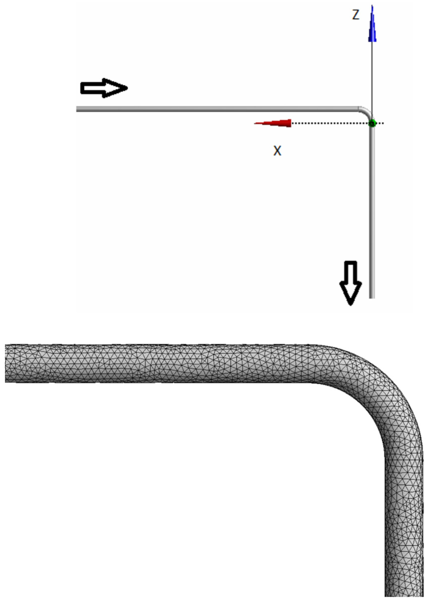
The arrangement of the flow system, with coordinates. Absent from the figure is axis y, which is normal to the figure plane. The fluid flows into and out of the pipeline at the points indicated by the arrows. A grid view of the pipeline is also depicted.

This literature review will focus solely on investigations of curved pipe flows. Research by Ito ⁴ focused on analysis of data concerning declining pressure during turbulent flow in smooth-pipe curves. Pipe bends of varying angle were attached to linear piping, to form a consistent entrance and exit flow. Laser-Doppler data were acquired by Enayet et al., ⁵ by assessing a 90° pipe curve’s laminar flow characteristics, where the pipe’s cross-sectional profile had a curvature of δ = 0.18. At 0.58 diameters prior to the curve inlet plane, the cross-stream plane was quantified with a Reynolds number of 500. Consistent laminar flow through a 90° pipe curve was also the concern of Van de Vosse et al., ⁶ who adopted a finite element method. The pipe’s cross-sectional profile had a curvature of δ = 0.17. The Reynolds number measurements fluctuated from 100 to 500. The curved section’s entrance and exit pipes were particularly short, with length one elbow diameter. The most contemporary investigation to date on curved pipe flow characteristics is that by Spedding et al., ⁷ who discovered that 90° bend flow characteristics were multifaceted. They determined therefore that developing a theory which reflected the practical dynamics is awkward, given the various flow features at the boundary and separation layers. Laminar flow in piping with a 90° bend, of a dilatant non-Newtonian fluid, was the subject of Marn and Ternik’s ⁸ research. In curved pipes with 180° bends, the excess pressure drop and the excess entropy generation bring forth serious penalties. To overcome these difficulties, a new partially curved pipe consisting of three straight pipe segments connected with two 90° bends was investigated in Hajmohammadi et al. ⁹ It was shown that the new curved pipe is advantageous because the pressure drop and entropy generation are considerably reduced. In Kim et al., ¹⁰ it was shown that new characteristic parameters can be used to represent the flow development in helical pipes. The development of friction factor and flow pattern along with the characteristic parameters was not significantly affected by the variations in Reynolds number, dimensionless pitch or curvature ratio at a given condition of modified Dean number and inlet velocity profile. The development of the friction factor was investigated in a modified Dean number range of 20–400, and a new correlation for the fully developed angles of laminar flows in helical pipes was proposed.

This assessment of the existing research indicates that understanding of 90° pipe bend flow characteristics is lacking, probably with as yet undiscovered dynamics. This is indicated particularly by Spedding et al.’s research. Therefore, this investigation seeks to contribute to a fuller understanding of the subject.

The mathematical model and numerical code

In a 90° pipe bend as expressed in Figure 1, the complete equations comprising Cartesian coordinates for flow are as follows:

• Continuity equation

  $$\frac{\partial u}{\partial x}+\frac{\partial v}{\partial y}+\frac{\partial w}{\partial z}=0$$
  (1)

• x-momentum equation

  $$u\frac{\partial u}{\partial x}+v\frac{\partial u}{\partial y}+w\frac{\partial u}{\partial z}=-\frac{1}{\rho }\frac{\partial p}{\partial x}+\upsilon \left(\frac{{\partial }^{2}u}{\partial x^2}+\frac{{\partial }^{2}u}{\partial y^2}+\frac{{\partial }^{2}u}{\partial z^2}\right)$$
  (2)

• y-momentum equation

  $$u\frac{\partial v}{\partial x}+v\frac{\partial v}{\partial y}+w\frac{\partial v}{\partial z}=-\frac{1}{\rho }\frac{\partial p}{\partial y}+\upsilon (\frac{{\partial }^{2}v}{\partial x^2}+\frac{{\partial }^{2}v}{\partial y^2}+\frac{{\partial }^{2}v}{\partial z^2})$$
  (3)

• z-momentum equation

  $$u\frac{\partial w}{\partial x}+v\frac{\partial w}{\partial y}+w\frac{\partial w}{\partial z}=-\frac{1}{\rho }\frac{\partial p}{\partial z}+\upsilon (\frac{{\partial }^{2}w}{\partial x^2}+\frac{{\partial }^{2}w}{\partial y^2}+\frac{{\partial }^{2}w}{\partial z^2})$$
  (4)

where y denotes the coordinates for the vertical, while coordinates for the horizontal are expressed by x and z. $\upsilon$ represents kinematic viscosity of the fluid; ρ denotes fluid density; u, v and w indicate the respective velocities and p represents pressure. Berger et al. ¹ and Van de Vosse et al. ⁶ both indicated that flow characteristics are impacted by the Reynolds number, extent of curvature and the Dean number. These three non-dimensional factors are indicated as

$$\mathrm{Re}=\frac{u_{m}D}{\upsilon }$$

(5)

$$\delta =\frac{r}{R}$$

(6)

$$\mathrm{Dn}=\mathrm{Re}\sqrt{\delta }$$

(7)

where $u_m$ expresses the average streamwise velocity, while D denotes the diameter of the bend. R represents the bend axis’ curvature radius, while r signifies the radius of the bend. Viscous, inertial and centrifugal influences are factored in by the Dean number, which was proposed by Dean ¹¹ in 1927 in relation to his research on pipe bend flow dynamics.

The dynamic software tool ANSYS Fluent 12.0 was utilised for numerical study and analysis. A steady-state, three-dimensional (3D) laminar solver was opted for alongside a third-order Monotonic Upstream-Centred Scheme for Conservation Laws (MUSCL) scheme for the momentum equations’ convective terms. The coupled scheme was chosen for the pressure–velocity coupling method. Continuity residuals, alongside x-, y- and z-velocity components, were all governed by a 10⁻⁸ criterion for convergence, while a double-precision degree of accuracy was opted for. ANSYS Fluent is a computational fluid dynamics (CFD) modeller which has been widely adopted in and tested through previous research, consequently its reliability and applicability to this research are well proven.

Figure 1 presents the set boundary conditions, as modelled by the ANSYS Fluent program. Three million cells were utilised in the pipeline. In Figure 2, the grid at the bend inlet and bend outlet is shown. There was a substantial entry pipe 100D in length, with an outlet pipe of the same size. The entry pipe had a consistent velocity as well as a boundary condition termed ‘velocity inlet’; the outlet pipe had a boundary condition termed ‘pressure outlet’. In Table 1, a grid independence test is presented showing that the three million cells utilised were enough in order that the results are grid independent.

Figure 2.

Grid at the bend inlet (left) and bend outlet (right).

Table 1.

Grid independence test for $\delta =0.2$ .

Reynolds number	Dean number	Number of cells	Friction factor
100	44.72	2,500,000	0.7558
100	44.72	2,800,000	0.7584
100	44.72	3,000,000	0.7586
1000	447.2	2,500,000	0.1269
1000	447.2	2,800,000	0.1297
1000	444.2	3,000,000	0.1302

Findings and discussion

Six varied curvature values $(\delta )$ were tested and data garnered from the results. By testing $\delta$ across a varied set of minor to very significant degrees, a thorough assessment of the effect of pipe curvature on fluid flow dynamics was undertaken. The non-dimensional parameter data are outlined in Table 2.

Table 2.

Non-dimensional parameter data.

$\delta$	Re	Dn
0.05	1–2000	0.22–447
0.067	1–2000	0.26–518
0.10	1–2000	0.32–632
0.20	1–2000	0.45–894
0.50	1–2000	0.71–1414
0.77	1–2000	0.88–1755

A Reynolds number of 2000 or less indicates that laminar flow is maintained. To ensure the validity of the model prior to its application, it was checked against previous research findings. Enayet et al. ⁵ had obtained Laser-Doppler data for laminar flow in a pipe’s 90° elbow bend with curvature $\delta =0.18$ . As indicated by Figure 1 in their research, the linear entry pipe’s length was proportionate to 5D, while the linear exit pipe’s length was proportionate to 10D. The pipe bend was static in the horizontal plane. Their quantifiable data were collected at 0.58 diameters from the bend inlet plane, in the cross-stream planes, with a Reynolds number of 500. Their data for experimental velocity were contrasted with this research’s quantifiable data, as laid out in Figure 3. It was determined that the validity of this research’s results was ascertained through the comparative assessment. There were some discrepancies between the two data sets, however there are two main explanations for this. First, Enayet et al. acknowledged that there might have been a degree of up to 5% inaccuracy in the quantifiable data obtained. Second, different bend diameters were used by this research and by Enayet et al. ⁵ The entry tube in their research was 5D, while for this investigation the entry tube measured 100D. With the accuracy of this study adequately assessed, its findings are now outlined below.

Figure 3.

Graph depicting the streamwise velocity at 0.58D upstream of the 90° pipe bend inlet, when δ = 0.18 and Re = 500.

Profiles of velocity

Each velocity profile outlined in this research relates to the horizontal middle plane. Presented in Figure 4 are the streamwise velocity profiles for various Reynolds numbers, at the bend entry in a pipe with δ = 0.77. The local streamwise velocity to average velocity ratio formed the non-dimensional velocity U in each instance. Increasingly wider velocity profiles resulting from rising Reynolds numbers led to a decline in maximum velocity. In addition, it is seen that the velocity profiles shift towards the inner side of the pipe. However, maximum velocity approached the value of 2 when the Reynolds number was diminished at the bend inlet. When a laminar flow’s profile is entirely parabolic in a linear pipeline, 2 is its extreme theoretical value. Figure 5 expresses the velocity profiles for various Reynolds numbers, at the bend outlet in a pipe with δ = 0.77. The velocity profile maintained its presence on the inside edge of the pipe bend when the Reynolds number was decreased. However, the velocity profile altered to the pipe bend’s outside edge when the Reynolds number was higher. As this happens, maximum velocity also decreased. The velocity profiles shifted to the outer edge of a pipe bend in this research is consistent with the findings of existing studies, as indicated by Figure 4 in Van de Vosse et al. ⁶ and Figure 5 in Marn and Ternik. ⁸ However, this investigation has revealed a further two dynamics that were previously unknown. First, the velocity profile of the fluid at the entry of the bend nearly matched that at the outlet, when there was a significantly small Reynolds number. This indicated that the fluid was flowing as it would in a linear pipe, with the bend’s impact on flow negated by the small Reynolds number. The second characteristic is the fact that at the same cross section some velocity profiles are shifted towards the outer wall and some towards the inner wall. Streamwise velocity profiles for the linear piping emanating from the bend outlet, when Re = 1000, are presented in Figure 6. It clearly indicates that velocity profiles were significantly altered between the point at the bend outlet and 1D further down the outlet pipe. The data indicate that there were two minima and three maxima, at z/D = 1. For the velocity profile to alter to such a significant degree in such a short length of space is peculiar. A parabolic shape in the velocity profile was achieved at 100D from the bend outlet, with local minima and maxima gradually diminishing up to this point. Figure 7 indicates the various velocity profiles at different distances down the outlet piping pertaining to a Reynolds number of 100, to determine the latter’s impact on velocity profiles. In the linear outlet piping, the progression of velocity profiles down the pipe contrasts somewhat to Re = 1000. There are no minima and maxima, with parabolic shape achieved in the velocity profile by 10D. Thus, we can determine from Figures 6 and 7 that a shorter distance is required for a return to regular parabolic shape, the smaller the Reynolds number.

Figure 4.

Velocity profiles at the bend inlet for curvature δ = 0.77 and different Reynolds numbers.

Figure 5.

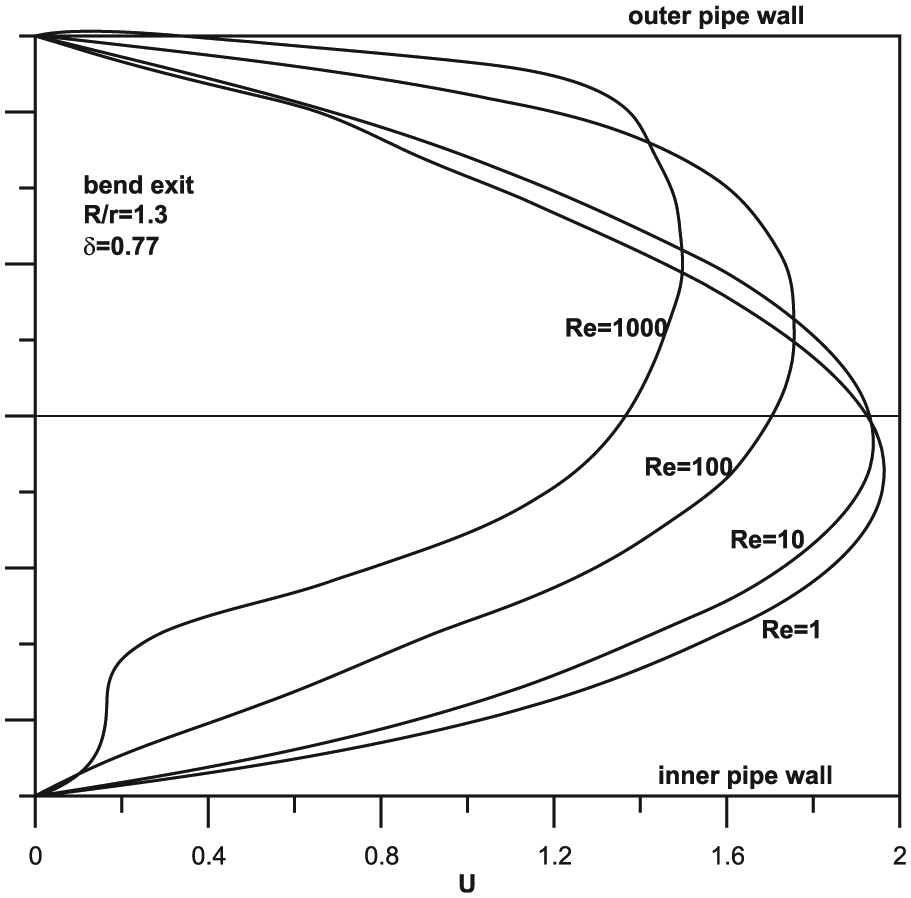
Velocity profiles for each Reynolds number with δ = 0.77, calculated at the bend exit.

Figure 6.

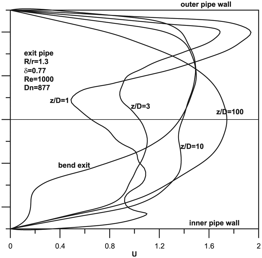
Velocity profiles after the bend exit at set points down the outlet pipe with Re = 1000 and δ = 0.77.

Figure 7.

Velocity profiles along the exit pipe at different distances from the bend exit for curvature δ = 0.77 and Re = 100.

Regarding flow in a more gradually curved pipe bend, streamwise velocity profiles for various Reynolds numbers at the bend entrance and bend outlet in a pipe with δ = 0.05 are shown in Figures 8 and 9, respectively. At the entrance to the bend, velocity profiles moved neither towards the outside nor inside pipe edge, maintaining a regular shape. This symmetry was maintained at the outlet when there was a small Reynolds number; however, asymmetrical velocity profiles were found, with a movement towards the outsider pipe edge, when there was an increased Reynolds number. Figure 10 presents the various velocity profiles down the outlet piping at set points, where it can be seen that parabolic flow is soon achieved, with no minima or maxima present.

Figure 8.

Velocity profiles for each Reynolds number with δ = 0.05, calculated at the bend inlet.

Figure 9.

Velocity profiles for each Reynolds number with δ = 0.05, calculated at the bend outlet.

Figure 10.

Velocity profiles after the bend exit at set points down the outlet pipe with Re = 2000 and δ = 0.05.

Dean vortices

In a pipe bend, additional flow dynamics are created by the main centrifugal force of laminar flow, comprising two counter-rotating Dean roll-cells. Dean^11,12 had proposed an explanation of this additional flow event. Centrifugal volatility at the outside edge of piping, caused by an increased Dean number, can cause Dean vortices to form, comprising a counter-rotating vortex pair. There are significant dissimilarities between Dean roll-cells and Dean vortex pairs, the primary one being the mechanics behind their formation. As in a space confined on each side by panels of varying higher temperatures, there is a disparity between viscous and centrifugal forces in the pipe, regardless of the Dean number, leading to the formation of Dean roll-cells. However, Dean vortex pairs are formed once an instability threshold and particular Dean number is passed, analogous to Rayleigh–Benard convection, making it a consequence of a particular instability effect. In figure 1 of Mokrani et al.’s ¹³ study, diagrams are presented of Dean vortex pairs and Dean cell pairs.

Alongside the velocity profiles, Dean vortex pairs and Dean cell pairs have also been determined for this research. The Dean number threshold, after which dean vortex pairs form, has been determined for the various degrees of curvature listed in Table 2. The process composed of calculating both the velocity streamlines and flow field at various planes in the pipe’s linear and curved sections, repeating the process for each set of Dean number and curvature. The amount of vortex pairs was the factor which decided the Dean number threshold. A small Dean number denoted that the single Dean cell pair would be present, however with a rising Dean number, additional Dean vortex pairs began to form.

Figure 11 presents the streamlines at δ = 0.2, Dn = 447 and Re = 1000, although the pattern was replicated across all the curve values. Figure 11(a)–(c) shows the streamlines along the bend at 30°, 45° and 60° angles from the bend inlet. It is seen that only Dean cells are formed at 30° cross section. Two more vortices tend to appear at 45° cross section (Figure 11(b)) and the two more vortices appear clearly at 60° cross section (Figure 11(c)). These extra vortices disappear at the bend exit (Figure 11(d)) and only the Dean cells appear here. Figure 11(e) indicates that within a brief distance down the outlet pipe, four vortex pairs were present, with three dean vortex pairs and the typical Dean cell pair shifted leftward. Further down the exit pipe, as presented in Figure 11(f), there are two Dean vortex pairs, with the Dean cell pair disappearing. Figure 11(g)–(i) shows the transition to one vortex pair, eventually disappearing altogether as the fluid flows through the outlet pipe. An original observation in this research, one which has not been noted in existing studies, was the presence of Dean vortex pairs in a linear pipeline. Between three to eight Dean vortices and Dean cells were present. The critical value of the Dean number for each $\delta$ value is shown in Table 3. The areas in which the Dean vortex pairs and Dean cell pairs formed are indicated in the bifurcation diagram (Figure 12). A similar bifurcation diagram has been presented by Yanase et al. ¹⁴ which concerns a continuously curved pipe without straight pipes upstream and downstream from a curved section.

Figure 11.

Streamlines for δ = 0.2, Re = 1000 and Dn = 447. The streamlines have been taken at different planes (cross sections) along the bend and exit pipe downstream from the bend exit. The origin of the z-axis lies at the bend exit. (a) cross section at 30° angle, (b) cross section at 45° angle, (c) cross section at 60° angle, (d) bend exit –z/D = 0, (e) z/D = 0.35, (f) z/D = 1, (g) z/D = 3, (h) z/D = 4 and (i) z/D = 16. In the above non-dimensional distances, the z is negative but its positive value has been considered.

Table 3.

Critical Dean number values for different curvature values.

$\delta$	Dn
0.05	447
0.067	258
0.10	158
0.20	179
0.50	212
0.77	263

Figure 12.

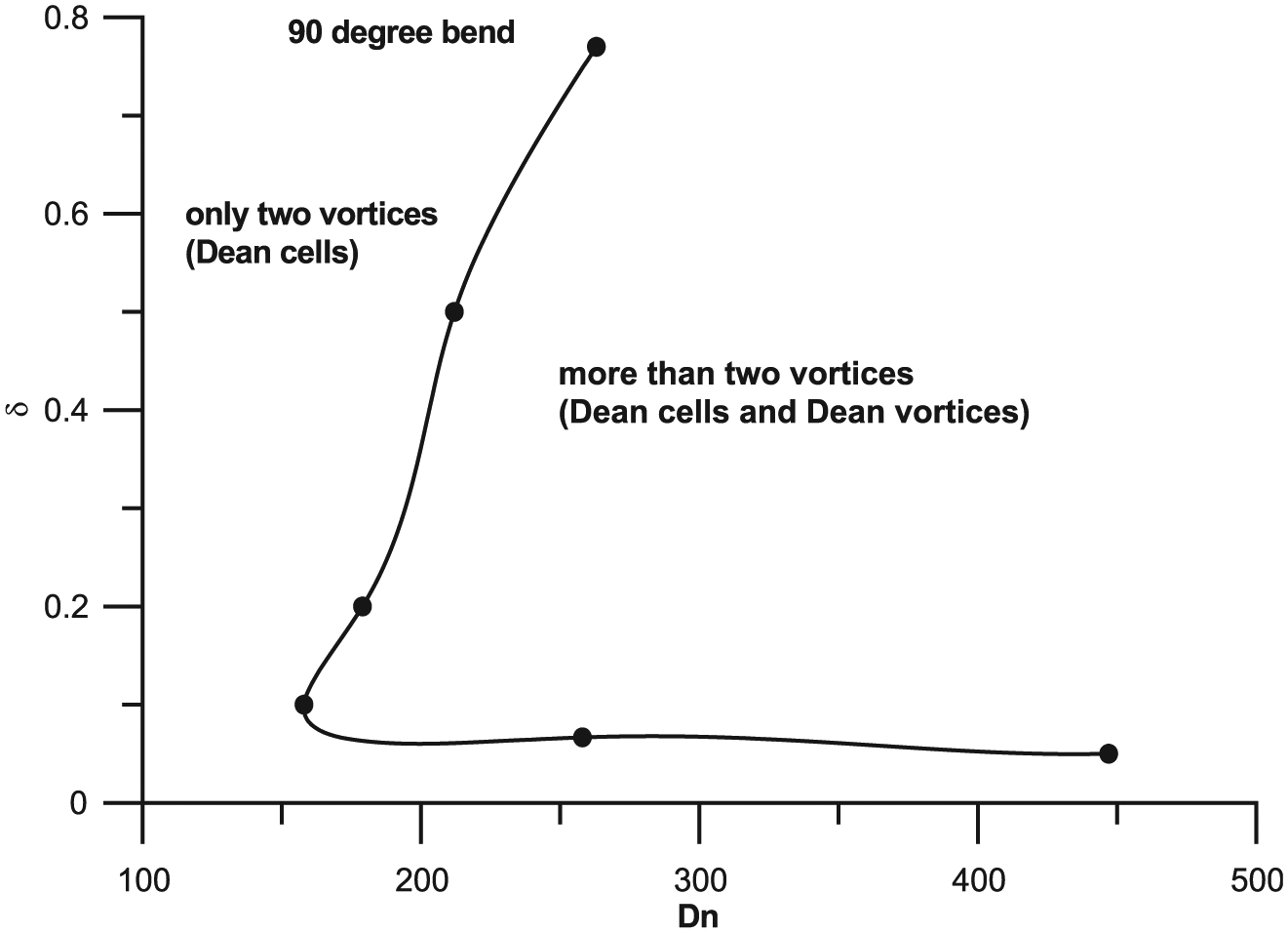
Areas where Dean cell pairs and Dean vortex pairs were formed, depicted on a bifurcation diagram.

Pressure loss and friction factor

Ito’s ⁴ investigation into declining pressure in turbulent flow through smooth-pipe bends was noted at the beginning of this article. Nevertheless, declining pressure in laminar flow through 90° pipe bends has not received a similar assessment. For varying Reynolds numbers between Re = 1 and Re = 2000, as well as for each $\delta$ value, the pipe bend’s Darcy–Weisbach friction factor and declining pressure were assessed. The Darcy–Weisbach equation is

$$\Delta p=f\frac{L}{D}\frac{\rho u_m^2}{2}$$

(8)

Bend axis length is represented by L. Figure 13 presents the Darcy–Weisbach friction factor for different bend curvatures, while the results for the smallest and largest $\delta$ values are presented in Table 4.

Figure 13.

Darcy–Weisbach friction factor for different bend curvatures.

Table 4.

Smallest and largest $\delta$ values’ Darcy–Weisbach friction factor results.

$\delta =0.77$			$\delta =0.05$
Re	Dn	f	Re	Dn	f
1	0.877	61.91	1	0.2236	64.59
10	8.77	6.37	10	2.24	6.46
20	17.54	3.39	20	4.47	3.23
100	87.70	1.0501	100	22.36	0.6786
500	439	0.6508	500	111.8	0.1839
1000	877	0.6238	1000	223.6	0.1100
1500	1316	0.6164	1500	335	0.0818
1800	1579	0.6418	1800	402	0.0717
2000	1755	0.6516	2000	447	0.0665

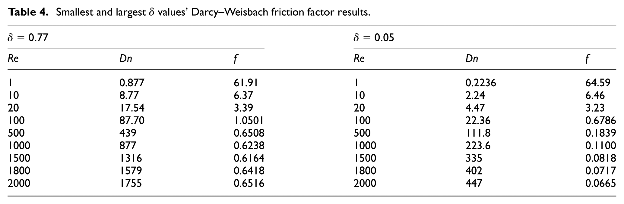
The Darcy–Weisbach friction factor can be considered as unaffected by the $\delta$ value when the Reynolds number is small, more reflective of the friction factor seen in a linear pipeline. When the Reynolds number increases, the friction factor is increasingly related to the Re, with a heighted friction factor also resulting from a larger $\delta$ value. A notable characteristic when $\delta =0.77$ , denoting a considerable curve degree, is that between Re = 1000 and Re = 2000 the rate at which the friction factor declines is slowed and plateaued out, in fact raising slightly at Re = 2000.

Summary of findings and concluding points

This research analysed the issue of 90° pipe bend laminar flow, with linear inlet and outlet pipers into the bend. The conclusions of the research are as follows:

1. When the bend curvature is high, the velocity profiles at the bend inlet are shifted towards the inner pipe wall, whereas at low curvature the velocity profiles remain symmetric.

2. At low Reynolds numbers, the flow passes through the bend without any change in the velocity independent of the bend curvature.

3. When the curvature is high, at the bend exit, the velocity profiles are shifted towards the outer wall at high Reynolds numbers and towards the inner wall at low Reynolds numbers. When the curvature is low, all velocity profiles are shifted towards the outer wall at the bend exit.

4. When the curvature is high, the velocity profiles along the exit pipe downstream of the bend show maxima and minima but this behaviour does not exist in the cases of low Reynolds numbers and low curvatures. In all cases, the velocity profiles become parabolic downstream.

5. The critical Dean number has been calculated for each curvature, and a bifurcation diagram has been produced showing the regions where the Dean cells and the Dean vortices appear. The Dean vortices start to form inside the bend, appear completely in the straight exit pipe and disappear at long distances from the bend exit.

6. The Darcy–Weisbach friction factor has been calculated and a diagram has been produced for the calculation of friction factor.