
Abstract
During the lifetime of a component, microstructural changes emerge at its material level and evolve through time. Classical empirical degradation models (e.g. Paris Law in fatigue crack growth) are usually established based on monitoring and estimating well-known direct damage indicators such as crack size. However, by the time the usual inspection techniques efficiently identify such damage indicators, most of the life of the component would have been expended, and usually it would be too late to save the component. Therefore, it is important to detect damage at the earliest possible time. This article presents a new structural health monitoring and damage prognostics framework based on evolution of damage precursors representing the indirect damage indicators, when conventional direct damage indicator, such as a crack, is unobservable, inaccessible, or difficult to measure. Dynamic Bayesian network is employed to represent all the related variables as well as their causal or correlation relationships. Since the degradation model based on damage precursor evolution is not fully recognized, the methodology needs to be capable of online-learning the degradation process as well as estimating the damage state. Therefore, the joint particle filtering technique is implemented as an inference method inside the dynamic Bayesian network to assess both model parameters and damage states simultaneously. The proposed framework allows the integration of any related sources of information in order to reduce the inherent uncertainties. Incorporating different types of evidences in dynamic Bayesian network entails advance techniques to identify and formulate the possible interaction between potentially nonhomogenous variables. This article uses the support vector regression in order to define generally unknown nonparametric and nonlinear correlation between the input variables. The methodology is successfully applied to damage estimation and prediction of crack initiation in a metallic alloy under fatigue. The proposed framework is intended to be general and comprehensive so that it can be implemented in different applications.
Keywords
Introduction
Structural health monitoring (SHM) exploits the condition-based maintenance (CBM) to avoid costly unscheduled and/or unessential repairs that are common in traditional time-based maintenance. 1 SHM uses CBM to continuously monitor the health state of the system via online sensors. In addition, SHM is closely related to nondestructive inspection (NDI) techniques which are usually carried out offline and with a priori knowledge of the damage locations. 2
The ultimate goals of systematic monitoring through SHM are prognostics and to predict the remaining useful life (RUL), which are essential for maintenance decision-making. RUL can be defined as the length from the current time to the end of the useful life of a component or a system. There has been an increasing interest in damage prognostics and estimating the RUL in recent publications with various outcomes and yet, there is still much room for improvement. Comprehensive reviews on monitoring and prognostics methodologies and applications can be found in Liao and Kottig 3 and Lee et al. 4
Notwithstanding the significant developments made by the current SHM in monitoring and prognostics for mechanical structures, most of the proposed methodologies in recent papers are established based on estimating conventional “direct damage indicators,” which are regarded as “observable markers of damage” in some studies, such as the fatigue crack size.1,5–8 However, by the time the usual inspection techniques efficiently identify the damage, majority of the life of the component would have been expended. 9 Moreover, there is always a possibility that such damage remains undetected and leads to catastrophic failures. Therefore, the main idea of this article is to establish a new SHM framework which is based on the “indirect damage indicators” referred to as “damage precursors (DPs).” Contribution of information content of DP into the traditional SHM frameworks provides a powerful platform to estimate the health state of a component/system even when direct signs of damage such as crack are not visible or measureable yet. Preliminary research in this area has been reported in Rabiei et al. 10
Damage estimation and prognostics in SHM are rooted in the filtering problem. The filtering problem, which involves estimating the state of a system that changes over time using a sequence of noisy measurements, has been around for quite a long time (almost since early 1960s). Different techniques, especially methods in the Kalman filtering family and the more advanced particle filtering (PF), have been proposed and implemented to address this problem. Unlike Kalman filter technique, which is applicable only to linear systems with Gaussian noise, PF does not require any restrictive assumptions and can provide a strong theoretical framework to address nonlinear models with non-Gaussian process/observation noise. Although application of PF in reliability field is quite new, 8 its popularity has increased rapidly in the recent years because of its flexible and powerful features. Other versions of the standard PF have also been proposed in the literature to improve the performance of the algorithm usually at the cost of more computation. Among them, one can refer to auxiliary particle filter, 11 regularized particle filter, 12 and unscented particle filter. 13 Researchers have used the standard PF algorithm and its variants for diagnostics and prognostics in many different fields such as life prediction of batteries and fuel cells (Dalal et al. 14 , Goebel et al. 15 , He et al. 16 , Miao et al. 17 and Jouin et al. 18 ), degradation assessment and prediction in gears and bearings (Yoon and He 19 , Zhou et al. 20 , Chen et al. 21 ), Health monitoring and prognostics of gas turbines (Sun et al. 22 ), machine tools (Wang et al. 23 ), and pumps (Daigle and Goebel 24 , Wang and Tse 25 ), and also, damage estimation and prediction of composite materials (Rabiei et al. 10 , Corbetta et al. 26 and Chiachío et al. 27 ). More application examples can be found in the most recent review paper on PF algorithm by Jouin et al. 28
However, most of the recent works in this area only consider one observation for updating the state estimations. For example, Wang and Tse 23 developed a prognostic method for estimating RUL of slurry pump impellers. They implemented the standard PF algorithm to assess the performance degradation of the pump impeller based on a moving-average wear degradation index. However, they only used vibration data both to develop the degradation index and to update the model. Similarly, Wang et al. 23 predicted the wear status of machine tools by recursively updating a physics-based wear rate model with online measurement through PF. They monitored the tool wear process via online measurements such as cutting force and vibration, and then they adopted statistical Pearson Correlation coefficient to select the most sensitive feature to tool conditions.
In addition, in the majority of the published works, measurements are exactly the same as the variable of interest and therefore, measurements can enter the PF algorithm directly only by adding some measurement noise. For instance, in the most recent work by Chiachío et al., 27 authors used PF to estimate the degradation of composite material which was defined as stiffness reduction and increase in matrix microcracks density. Then, they measured the same variables (microcracks density and stiffness) through the experiment and update the PF estimations. In a similar research by Corbetta et al., 26 a PF-based framework was proposed for predicting a structure’s RUL with consideration of multiple co-existing damage mechanisms of delamination and matrix cracks in composite. Again, although multi-states evolution was considered in the PF, the measurements were exactly the same as the variables of interest. However, most of the time, the variable of interest is hidden and the type of gathered measurements might be very different from the state of interest. For example, the length of a fatigue crack might be of interest, but acoustic emission (AE) waves and temperature variation near the crack are available instead. In such cases, it is more challenging to consider multiple measurements with different natures directly into the PF.
With recent advanced sensing and monitoring technologies, it is important to develop a framework which is capable of fusing various measurements and informative evidences from multiple sources and with different natures. Any piece of related information can be influential in reducing the inherent uncertainty and obtaining more robust and reliable predictions. Accordingly, the idea of this study is to integrate multiple evidences that might be very different in nature. Dynamic Bayesian network (DBN) 29 has been recognized as one of the powerful approaches to deal with the correlation of complex time-dependent and uncertain variables.10,30–32 And, PF is one of the most effective and flexible stochastic filtering techniques that can be applied to make inference inside the DBN. Therefore, in this article, the PF is utilized as an inference method in DBN when multiple measurements are to be integrated.
One of the difficulties in applying DBN to real-world application is the challenge of defining the causality and/or correlation between variables. In order to make inference in DBN, the relation of all the related variables should be identified through physical, empirical, data-driven modeling, or based on expert-elicitation models. Although physical models surpass other types of models, 33 understanding the underlying physics of failure and its relation with other sources of evidences are not always feasible, especially when dealing with less explored areas such as DP. Therefore, this article applies more advanced and flexible data-driven machine learning models, that is, support vector regression (SVR) 34 in DBN/PF framework to address this challenge.
Lastly, in this article, damage evolution is investigated in samples of aluminum alloy specimens under fatigue test. The article shows how the proposed SHM framework is applied to a real case study to estimate and predict the damage accumulation in the component before crack initiation. The methodology relies on monitoring the variation of DP during the experiment and integrating any other available evidence to infer the underlying degradation state.
Damage precursor
There is no unique and universal definition for DPs. The interpretation of DP might vary based on the field and type of damage itself. Weiss and Ghoshal 35 defined DP as the progression of structural material property degradation or morphology that can evolve into damage. This description implies that DP in this context is some microstructural changes that happen “before” damage and can “develop into damage.” However, this notion depends on definition of damage itself. The concept of damage is somewhat abstract, and its definition relies on the field variables used as damage indicators or markers of damage to describe the anticipated aging or degradation process36,37. In fact, definitions of damage due to physical mechanisms vary for different materials, geometries, and scales. Therefore, deterioration of microstructural properties—which is called “damage precursor” by Weiss and Ghoshal 35 —itself can be regarded as damage of the component at microscale, although common NDI techniques might not be able to capture it. Therefore, a broader definition of DP is needed to convey the idea. Accordingly, we extend the definition of DP to “any noticeable variation of material/physical properties of the component that informs about the evolution of the hidden/inaccessible/unmeasurable damage during the degradation.” In this definition, DP can refer to any indirect damage indicator that is revealed as a sign of microstructural changes and can describe the underlying degradation process when conventional direct damage indicators, such as crack, are not recognizable or accessible yet. In this article, DP and indirect damage indicator terms are used interchangeably.
Some microstructural changes, which are currently known as DP, are identified in laboratory settings for metals and composites under fatigue. They include increase in dislocation density, crazing, inhomogeneity of strain, shear localization, variation of electrical resistivity and conductivity, change in chemical composition, electrical signal, and acoustic response.10,38–43
The idea of considering DP in SHM frameworks10,44 provides the opportunity to estimate the damage state of a component when direct signs of damage (e.g. crack) have not developed yet or are difficult to measure (e.g. complex degradation processes in composites). Therefore, with the help of DPs, one can assess and ultimately predict the degradation state.
DBN approach to integrate various evidences
Prognostics—as the ultimate goal of SHM framework—inherently concern with significant uncertainty especially when dealing with a less explored area of researches such as DP-based SHM. The challenge in prognostics is that one desires to look into the future and make predictions of RUL with no additional evidence. Consequently, high level of uncertainty exists when performing long-term damage prediction. In order to reduce the uncertainty, the SHM framework should be able to integrate any piece of available evidence. Such evidences might have different natures and come from various sources.45–47 The SHM framework can benefit from useful information derived from online and offline monitoring data (collected from built-in sensors and NDI, respectively), partially relevant data (comes from similar systems but not necessarily identical to the target system), expert opinion, any other sources such as relevant published literature, reliability handbooks, and historical data.
Combining these various evidences might be tedious, so a flexible and powerful methodology is required to deal with inherent challenges. DBNs have been known as a powerful and suitable approach for integrating many different evidence types because of its following beneficial features:48,49
DBN facilitates the understanding of complex systems by providing a graphical representation of all the variables and their temporal and functional dependencies.
DBN framework enables us to consider different sources of uncertainty that might exist in the system such as measurement uncertainty, detection error, and modeling error. 6
DBN is capable of efficiently integrating information from different sources such as physical model, historical data, operational data, and expert opinions. 45
As soon as new evidence becomes available, DBN incorporates that information to update the belief state of all the variables. This feature makes it favorable in damage diagnosis and prognosis in time.
Therefore, in this article, DBN is adopted as the primary modeling technique to fuse the various evidences in order to reduce the uncertainty and obtain a more robust estimation.
Proposed methodology
The objective is to establish a SHM framework based on evolution of DP, considering different available sources of uncertain evidence. Consider a component/system in operation under load when a conventional direct damage indicator (such as crack length) does not exist, or is very small or difficult to detect. This article proposes a two-stage SHM framework (Figure 1) to estimate the health state of the component/system based on identifying and monitoring the evolution of a proper DP until the direct damage indicator is recognized. Then, when a direct damage indicator (e.g. fatigue crack length) becomes measureable by conventional NDI tools, the focus of the methodology can shift to tracking propagation of the direct damage indicator instead and implement the widely used empirical models such as the Paris Law. Otherwise, if necessary, health assessment can be continued based on the evolution of both DP and direct damage indicator.

Proposed two-stage SHM framework for monitoring and prognostics.
The criterion for prognostics and predicting the RUL is completely application dependent. For instance, in one case, the component might be considered as already-failed, as soon as the crack is initiated. Therefore, prognostic can be seen as predicting the “crack initiation time.” Whereas, in another case, component can be still operational until the crack size grows and reaches some specific threshold. The proposed DP-based SHM framework, Figure 1, tends to be general to represent both scenarios. In the following, the main elements of the proposed methodology are discussed in detail.
Stage I: Damage precursor modeling
The first stage is based on identifying and monitoring the evolution of the proper DPs. It requires a deep understanding of the possible failure mechanisms, system’s functionality, relevant components and their interactions, and other influential factors. As shown in Figure 1, stage I of the proposed framework consists of the following:
Identify the microstructural damage mechanisms for the material under consideration and in a particular application.
Look for a set of precursors that collectively represent the highest information content about the progression of the damage.
Monitor the material’s health state based on variation of DP.
Extract and quantify DP index; appropriate indicators are material and application dependent.
Develop a model for evolution of DP.
Stage II: direct damage indicator modeling
Microstructure defects grow over time and evolve into observable damage in the component. When a direct damage indicator is recognized and measured, one can switch the modeling approach to more traditional damage evolution models that already exist in the literature. For example, underlying physical mechanism of direct damage indicators such as crack has been widely studied and several models have been proposed including Paris Law, 50 modified Paris Law, 51 and Weertman’s 52 equation for fatigue crack growth. In order to incorporate this information into the SHM framework, we need to do the following:
Recognize widely known direct damage indicators such as crack and metal loss based on the dominant physical failure mechanisms.
Monitor and measure damage indicator with conventional NDIs.
Identify or develop an appropriate model that can represent the progression of damage through time based on influential agents (such as load, temperature) and model parameters.
Consider sources of uncertainty including model uncertainty and model parameters uncertainty.
Integrate other evidences
As seen in Figure 1, the idea of integrating all the other available evidences into the SHM framework is graphically represented by an independent box (middle top) that can feed into both stages of the framework.
Mathematical framework
As explained earlier, DBN is the main approach underpinning the proposed framework considering correlation among the variables and their uncertainties. Inference in DBN is not trivial especially when dealing with various evidences and unknown or partially known degradation model. Consequently, flexible filtering techniques such as PF would be very beneficial to perform the inference in DBN. In this section, the mathematical details of PF for state estimation along with joint particle filtering (JPF) for both state and parameter estimation are presented. Later on, the procedure of damage prognostics and prediction of time to failure (TTF) with JPF are explained. And finally, a brief introduction on SVR is presented to demonstrate how it fits into our mathematical framework.
Particle filtering
PF is a computational technique, also referred to as sequential Monte Carlo, which uses Bayesian recursive estimation to address the filtering problem especially when dealing with nonlinear and/or non-Gaussian processes. In the context of this article, suppose

where

xk is the state at the time step k,

where v is the measurement noise and h is the possible nonlinear function to link observations to states.
Weights of the particles
Joint estimation of model parameters and states in PF
The original PF is established based on the assumption that state process model is fully defined with fixed known parameters in advance. However, in many cases, even if the form of state model is known, all or some of the parameters might be unknown. This aroused an interest in combining parameters and states together and estimating both of them simultaneously.55–58 In this regard, the degradation process based on evolution of DP is not fully known in advance; therefore, in this study, it is required to learn the damage model by online tuning its parameters as well as estimating the damage states.
The extension of standard PF to a JPF is not trivial. One of the conventional proposed strategies is to treat the model parameters the same way as states, which results in estimating the augmented state space problem

where g and

The last term in equation (5) is the main modification in the posterior of the original PF and it should be estimated accordingly. It is suggested in Kitagawa
55
and Liu and West
56
that a Gaussian random walk with mean 0 and variance

Note that the parameters are not time variant, that is, they are not supposed to dynamically evolve in time. Therefore, adding random noise results in more diffused posterior relative to the theoretical posterior of the actual fixed parameters. This issue was recognized very early and an approach based on kernel smoothing was proposed by Liu and West
56
to control the variance. The idea of kernel smoothing is to reduce the variability in particles by shrinking them (with shrinkage parameter h) toward the current estimated mean

where m is the kernel location calculated for each particle (i) with the following shrinkage rule

The value of h ∈ [0,1] is suggested in Liu and West 56 and Chen et al. 59 to be less than 0.2 for slowly varying particles and more than 0.8 for highly stochastic process. Some works also have been published recently on optimizing the value of h using historical data or online observations.60–62
Consequently, selecting a JPF algorithm as an inference technique along with kernel smoothing for handling unknown parameters will make DBN more flexible and powerful to model complex nonlinear systems.
Prognostics with joint particle filtering
Prognostic with Bayesian recursive approaches such as JPF deals with the challenge of making long-term predictions without having any further observations to update the estimated states. Some methods are proposed in Zio and Peloni, 7 Orchard and Vachtsevanos, 8 and Liu et al. 63 to handle this issue. As shown by Orchard and Vachtsevanos, 8 the simplest approach that can provide satisfactory results is to keep the particle weights invariant during the long-term prediction. In this approach, the weights of the particles are updated based on the last available observations in the current time instance and then these weights are stored and kept constant during the long-term predictions.
Each weighted particle can be considered as a hypothesis of the hidden state (i.e. state of damage in this article), which we desire to estimate and also predict in future. Having a predefined threshold for damage,
Note that long-term prediction heavily relies on state process model. Since in JPF algorithm, the parameters of the state model are not known in advance and are supposed to be learned during the process, and the accuracy of prognostics depends on the state of convergence or maturity of the parameters at the time of prediction. Predictions cannot be reliable when variation in model parameters is still large.
Support vector regression
When a complex DBN is adopted to represent an unknown and complicated degradation process, the relationship between all the involved variables needs to be defined. Although a field expert would be necessary to learn the structure of the DBN and identify the possible links between the nodes, physical, empirical, or data-driven models are required to quantify such links. However, there might not be a proper predefined model to interpret the relationship between some of the variables. It is worth noting that the relationship between the nodes in DBN can be either based on causality or statistical correlation. In cases where underlying physical causality is missing or unexplored, more flexible techniques such as regression with support vector machine (SVM) can play an important role to define the possible correlation.
SVR 34 is an extension of a supervised machine learning technique called SVM which was originally developed by Cortes and Vapnik 64 for binary classification. SVR implements the nonparametric kernel-based method to model the relationship between input and output variables. Examples of successful application of SVR in different fields such as risk and reliability can be found in Moura and colleagues.65–67
SVR has flexible features that make it a very good candidate to perform regression to describe the relationship between some variables:
It is especially powerful to model generally unknown nonparametric and nonlinear mapping between input and output variables.
It is particularly useful when the underlying functional relationship between random variables is not fully known.
It does not require any hypothesis on the distribution of the variables.
It does not require any assumption on the distribution of noise.
It guarantees to find the global optimum.
However, There are some concerns related to the SVM and SVR such as being deterministic or using a lot of kernels to perform the regression/classification. Hence, recently in the literature, more sophisticated techniques such as relevance vector machine (RVM) 68 and bootstrapped SVR 67 have been introduced to remedy these concerns by proving uncertainty quantification via different approaches. Nevertheless, for the problem at hand, at this stage of the framework development, SVR presents promising results based on our experimental data. Therefore, SVR was implemented in this research to capture the relationship between some of the key variables in the DBN. Brief mathematical background of SVR is presented in the following.
Suppose we are given l pairs of observed data

where

The weight vector

Subjects to conditions

Therefore, the SVR equation for nonlinear predictions for the optimal value “o” becomes
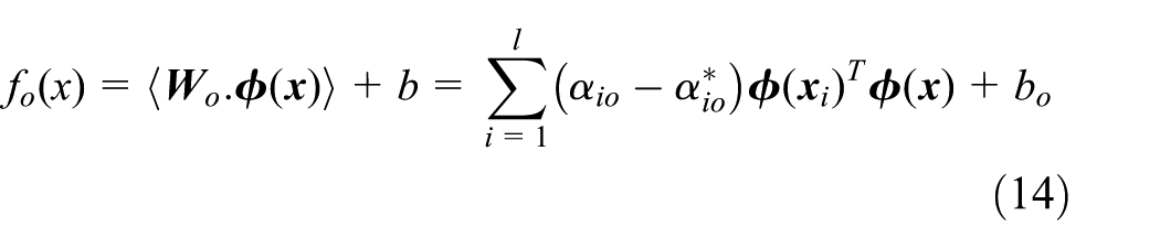
Regression with SVR is different from other regression techniques because of the term
In this article, SVR with RBF kernel function is implemented inside DBN to define the unknown nonparametric and nonlinear correlation relationships between some of the hidden and/or observed variables. The trained SVR then will be introduced into JPF algorithm to infer the model parameters and damage states.
Case study: monitoring and prognostics in metallic specimen under fatigue test prior to crack initiation
As described earlier, in many cases when a component is under load, unseen microstructural changes occur inside the component that gradually evolve into visible and measureable damage markers. Therefore, there is a time period when, although the component seems quite healthy and does not reveal any conventional recognizable damage signs, degradation is actively happening inside the component. The idea here is to be able to monitor the health of the component even when visible direct damage indicators such as crack do not exist.
Experimental setup
For this purpose, an accelerated life testing is designed and run in the Laboratory of the Center for Risk and Reliability at the University of Maryland, College Park. In this set of experiments, dog-bone 7075-T6 Aluminum samples undergo cyclic load with frequency of 5 Hz and stress ratio of R = 0.1. Samples contain a small notch in order to localize the stress intensity and accelerate the degradation process. Extension of the specimen is measured by extensometer which is placed around the notch area. Moreover, two AE sensors are also employed on the sample in order to capture any acoustic wave emitted during the fatigue test.
A high-resolution microscopic camera is adjusted and zoomed on the notch area that captures photos every 5 s. When setup is complete, the specimen experiences fatigue under cyclic load with maximum load of 11 kN. Experimental setup and schematic of the test specimen are shown in Figure 2.

Schematic dog-bone specimen used for the fatigue test (left) and experimental setup (right).
Defining the proper damage precursor
Since the focus of the experiment is on crack initiation, the test will be stopped as soon as the first signs of crack can be recognized by microscopic camera. Such experiment relates to the time period before crack initiation in the component, so conventional damage models (e.g. Paris Law) are not valid and cannot be applied to estimate the damage level. Therefore, without loss of generality and because of the nature of the experiment, only stage I of the proposed framework (Figure 1) can be employed in this case study. If the experiment were to continue after crack initiation into crack growth until some predefined threshold is reached, then stage II of the framework would be applicable as well.
Having experimental results, the challenge is to define DPs which can explain the microstructural degradation happening in the component prior to crack initiation. Referring to the proposed SHM framework in Figure 1, the procedure of state estimation starts in stage I by identifying the microstructural damage mechanisms and proper DP. When a component undergoes fatigue loading, microstructural changes such as micro-deformation, slipping, and microcracks at grain’s boundaries happen at material scale which can be treated as underlying damage mechanisms. Such phenomena, although unobservable, make the component weak and reduce its resistance to deformation. Modulus of elasticity, as the measure of substance’s resistance to deformation, has been reported in the literature74,75 as one of the microstructural properties that changes during degradation. Therefore, variation of modulus of elasticity can be considered as a DP that would provide insight about the undergoing damage within the component in advance to any visible crack on the surface of the component.
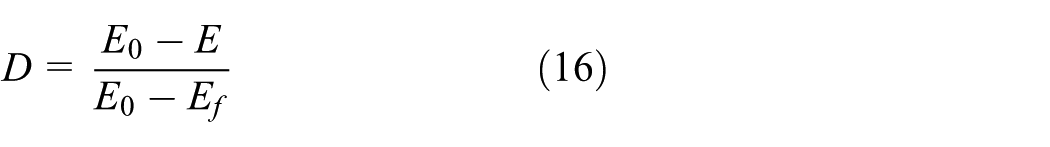
Lemaitre 74 proposed that it is possible to estimate the damage through the variations of the modulus of elasticity. If E0 is the modulus of elasticity of undamaged material, then damage parameter D can be expressed as follows

where E is the modulus of elasticity for the degraded material. As soon as damage occurs and propagates in the material, modulus of elasticity decreases. This relationship is simply presented in equation (15). In this model, damage would reach 1 only if E reduces to 0. This situation might not be obtained in reality, not even at breakage point. A modified version of the Lemaitre damage parameter74,75 was introduced by Mao and Mahadevan 76
where
Having defined a suitable DP, the next step is to monitor and quantify its variation (levels 3 and 4 in stage I of Figure 1). Modulus of elasticity is basically the slope of stress–strain curve in elastic region. Since we are dealing with cyclic load, stress–strain curves will form hysteresis loop throughout the loading process. Variation of stress–strain can be monitored by extensometer. To quantify E, the slope of the linear portion of stress–strain loop is calculated for each loading cycle in the hysteresis loop. Figure 3 shows how modulus of elasticity changes during the aforementioned experiment.

Variation of the modulus of elasticity during fatigue test prior to crack initiation.
DBN representation: general overview
Figure 4 represents the high-level DBN for modeling the degradation process in this experiment. As explained above, in the hidden layers of the material, damage mechanisms take place that result in change in modulus of elasticity, E. In this case, E can be measured and tracked through monitoring variations of hysteresis loop in each cycle. Calculated modulus of elasticity is then entered into equation (16) to acquire a normalized damage index D used as a proper representative of hidden damage evolution. On the other hand, AE sensors can capture signals from underlying progressive degradation. AE signals can be treated as observed evidence of hidden damage.
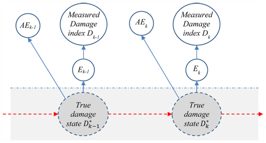
DBN representation of the damage evolution considering actual hidden underlying damage mechanisms.
Having the DBN topology ready, probability distribution of all the correlated nodes should be defined in order to make inference in DBN. Each arrow in Figure 4 indicates the probabilistic relationship between the nodes that need to be modeled by physical or data-driven methods. Hence, in the DBN shown in Figure 4, probability distributions
Inference in DBN using joint particle filtering
A combination of physics-based and data-driven models is required to represent the relationships between the nodes in the DBN in Figure 4. To make an inference about the hidden variables (true damage parameter D*) in the DBN, state process model and observation models need to be identified. The details are presented in the following.
Online learning of both state and parameters in the degradation model
Ideally, it is advantageous to apply physics-based model to describe the system degradation in the form of an analytical system equation (degradation model). The standard particle filter state estimation process was retained as the model-based technique. Mao and Mahadevan 76 proposed a versatile empirical model for explaining the evolution of damage index in composite material (see equation (17)). Although the model was first suggested for damage parameter in composites, the form of the model fits our experimental results very well. This is because of the two-part format of the model as the first term controls the damage accumulation at the beginning of the degradation, and the second term captures the fast damage growth toward the end of the life. Therefore, based on our experimental results, the model is quite satisfactory for explaining the behavior of damage evolution in terms of decrease in modulus of elasticity prior to crack initiation in our case study.

In this equation, q, m1, and m2 are model parameters that need to be estimated online during the experiment and n is the elapsed cycle which is normalized with respect to number of cycles at failure threshold Nf. However, in online monitoring of the component/system, the value of Nf is not known in advance. In fact, estimating the maximum number of cycles to failure is the final objective of the whole diagnostics and prognostics framework. Therefore, Nf is treated as another unknown model parameter that needs to be updated in real time.
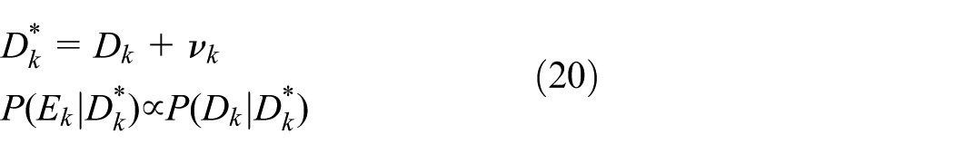
State of damage at each time step k relates to not only the elapsed cycle, but also to its previous damage level
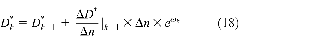
where

Equation (19) is used to describe the probability distribution
Observation model
Real-time observations will be used to weigh the projected particles. In this case study, two types of observation are available: one is AE signals and the other is the measurements of variation of modulus of elasticity E as DP. In order to demonstrate the importance of incorporating different observations into the framework, three cases are studied here:
Case 1: only consider AE signals, that is,
Case 2: only consider measured modulus of elasticity E, that is,
Case 3: consider both AE signals and measured modulus of elasticity, that is,
In case 1, the likelihood of observing AE signals at time step k given underlying damage state should be estimated. AE signal acquisition system captures and reports different features of AE signals. In this study, cumulative absolute energy of signals is calculated and employed as one of the observations. Ideally, in an online monitoring process, it is preferred to implement new observations as soon as they get available to update a predefined empirical or physical model. However, not all the time a well-defined physical or empirical relationship exists between the variables. To the best of our knowledge, there is no pre-determined model to correlate the cumulative absolute energy of AE signals to underlying hidden damage parameter prior to crack initiation. Moreover, no common type of regression family can efficiently model this relationship. Therefore, to overcome this challenge, more flexible regression approach based on SVM is applied. A SVR model is trained offline based on 60% of captured AE signals (Figure 5). This model, including some measurement noise

Correlation of damage index and cumulative AE energy using SVR (SVR model is trained based on 60% of data)
On the other hand, in case 2, we assume that only in-situ measurement of modulus of elasticity as indirect damage indicator prior to crack initiation is incorporated in the likelihood equation. Measured E will be used in equation (16) to calculate damage level D. Considering measurement uncertainties
Expert opinion and specification of measurement instruments (AE acquisition system and extensometer) are used to decide about the observation noises
And finally, in case 3, when both AE and E are available simultaneously, an integrated measurement model is required as

In this case study, it is reasonable to assume that variation of modulus of elasticity is independent of captured AE as they are different in nature; therefore,

More details on estimating these three cases as well as existing challenges are presented in the next section.
DBN representation: detailed model
Now that all the elements of the DBN and the details of state process and observation models are explained, a more elaborate version of Figure 4 can be constructed. Figure 6 demonstrates the detailed DBN of this case study.

Detailed DBN representation considering all the factors.
In Figure 6, observations (i.e. AE signals and measured DP E) are shown with rectangular box. Recalling from section “Inference in DBN using JPF,”
Results and discussion
In each case mentioned in previous section, 5000 particles that included 1000 particles for each variable (q, m1, m2, Nf, and damage states D) were randomly selected. Any prior information about the initial value of the parameters would be very helpful in achieving the faster convergence of the technique. Such prior information might come from related published papers, similar experiments, or expert opinion. In our case, the suggested range 76 for parameters m1 and m2 are m1 < 1 and m2 > 1. However, more information on the value of the parameters was obtained from fitting the same model to other experiments under similar test conditions. Therefore, model parameters were initialized as follows: q = uniform [0.01, 1], m1 = uniform [0.1, 0.8], m2 = uniform [18, 25] and Nf = uniform [10,000, 14,000]. Also, for damage states D, initial particles should be selected very close to zero as it is assumed that the component is completely healthy and no damage exists in the component before loading. Randomly selected particles are propagated in time based on the proposed state model with unknown model parameters, equation (19), following the procedure explained in section on JPF. The estimation of the model parameters as well as states will be updated once any measurement gets available. The methodology will be validated by comparing the estimation and prediction results of DBN with the true damage evolution. The following results present that the proposed methodology is able to effectively track the true damage evolution based on variation of modulus of elasticity along with captured AE signals.
Damage state monitoring
In case 1, when only one observation model exists

Estimation of damage evolution in time using (a) only AE signals, (c) only measured E, and (e) both of the evidences. Right graphs (b, d, and f) show the corresponding model parameters.
In case 2, however, modulus of elasticity can be measured in each cycle; therefore, there will be plenty of observations to both learn the model parameters and estimate the damage state. Measurement model
Figure 7(e) shows the results of damage estimation in case 3 when both AE signals and E are incorporated in the DBN for the updating process. It was noted that results were improved and more precise estimation was achieved. It is interesting that although AE signals seem to be very ineffective and incapable for updating the states and parameters when used alone in case 1, they can improve the results when combined with E measurements. Compared to cases 1 and 2, DBN approximations of damage state in case 3 follow the trend of true damage evolution more accurately through time, and even the uncertainty of estimation (dispersion of particles) was reduced especially at the tail where many AE signals are available.
Since the observations (AE signals and E measurements) are not necessarily synchronized, they do not enter into the DBN simultaneously. Therefore, the procedure for considering both evidences is as follows: as soon as any of the observations (AE signals or E) arrives independently, the model parameters and damage state are updated with corresponding measurement model similar to cases 1 and 2. And if both AE and E were captured simultaneously, then equation (21) should be used to consider the fused measurement model.In other words, unlike regular filtering techniques, in this approach time step
Another important improvement in fusing different observations is illustrated in convergence of model parameters. Figure 7(f) shows the smoother and more stable convergence in all the model parameters q, m1, m2, and Nf. This feature is especially significant in prognostics. Since in dual updating PF algorithm, model parameters are not known in advance, prognostics results are not reliable unless fluctuations of model parameters subside.
Prognostics and crack initiation prediction
Without loss of generality, suppose that at a particular time Tp, one intends to look p step ahead and predict the RUL. In this case study, the experiment stops immediately after detection of crack by the optical camera. Therefore, RUL here relates to remaining life before the crack initiation, and prognostics corresponds to predicting the crack initiation time. As explained earlier, prognostics in JPF algorithm is more challenging, because not only no other observation exists to update the estimation, but also the degradation model itself is not fully known. Therefore, prognostics should be postponed until variation of model parameters decreases.
Figure 8 shows the result of prognostics at Tp = 4000 cycles. E measurements and AE signals were employed to learn the model parameters and damage states (like case 3) up to 4000 cycles and after that no more observation was collected. Prognostic was performed by propagating the particles in time relying only on state process model without any more updating in model parameters and/or states. It is evident that in this case, the particles disperse more and more through time. However, the final approximation of PF (

DBN prediction of damage evolution, starts at 4000 cycles until crack initiation (left) and variation of model parameters (right). Model parameters do not change during prognostics.
Prediction of the TTF and RUL, as the ultimate goal in prognostics, is based on a predefined damage threshold. Characterizing the failure threshold depends on the features of the problem in hand. In our case study, “failure” relates to observing first signs of direct damage indicator (crack initiation), so TTF means time to crack initiation. In that sense, the threshold in this study is defined as evolution of damage parameter reaches 1.
As described in the section “Prognostics with JPF,” each particle is tracked from the start of prognostics (Tp) until it passes the threshold at cycle tf. The process continues until all the particles cross the limit and fail. The TTF corresponds to a distribution over all the

Long-term prediction of the TTF using DBN.
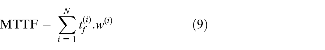
Referring again to Figure 7(f), it can be seen that although variation of model parameters decreases after 4000 cycles, there is still some noise especially in parameters m1 and Nf. So, it is expected to get different prediction results if the prognostics begin at different cycle Tp. In order to show how the accuracy of the prognostics will change with respect to variation of parameters, the prognostic procedure was repeated with different starting points namely 4000, 4200, 4400,…, 7000 cycles. The noise in the model parameters at the aforementioned prediction starting times Tp results in slightly different distributions for TTF (shown in Figure 10). However, the average of their MTTF is 11,415 cycles which is in 0.2% error with respect to true TTF = 11,444 cycles. The true TTF is when crack initiation is detected by the microscopic camera and the experiment stops.
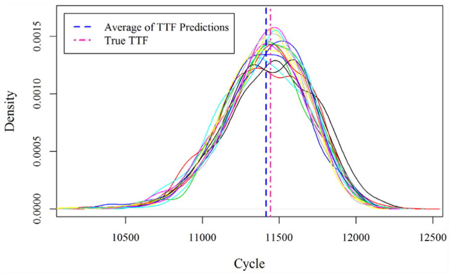
Different distributions of TTF when prediction is done at different cycles in (4000, 4200, 4400,…, 7000).
Conclusion and future improvements
In this study, a new SHM framework was proposed based on monitoring and estimating the evolution of DPs when conventional direct damage indicators such as crack is unobservable, inaccessible, or difficult to measure. It is shown that unlike traditional widely used empirical damage models (such as Paris Law), the proposed framework does not have to wait until a known direct damage indicators such as a fatigue crack is observed, whereas it is able to inform about the underlying damage much earlier by monitoring the evolution of some predefined DPs. Hence, there would be more time for decision-makers to perform corrective actions. The proposed framework is intended to take advantage of various sources of available information in order to reduce the inherent uncertainty and achieve more precise estimation of the system’s health state. DBN was adopted as the main modeling technique to materialize the proposed SHM framework.
To demonstrate and validate the proposed approach, the results of a fatigue test on Aluminum specimen prior to crack initiation were used. A model based on variation of modulus of elasticity E as a DP was developed to describe the underlying active damage state in the component while crack had not emerged yet. A DBN was established to represent the related variables and their causal or correlation relationships. Since the degradation model based on DP was not completely known, the model parameters also needed to be learned during the monitoring process. JPF along with kernel smoothing technique was applied to infer both the model parameters and the damage state in the component prior to crack initiation. SVR technique, which is a powerful and flexible method especially for describing an unknown nonlinear correlation, was also implemented inside the DBN to incorporate AE signals. The results of the proposed framework in real time estimating the damage state are in good agreement with the experimental observations. Consequently, the methodology described in this article was able to successfully track the true damage evolution and predict the crack initiation when no direct damage indicator existed. Moreover, the article showed how incorporating various observations in the framework leads to more precise estimations and predictions. Also, integration of different computational approaches (i.e. DBN, JPF with kernel smoothing, and SVR) in the present framework provides a more general and flexible methodology that can be applied in many different case studies. Although the current results of the proposed framework are promising at this stage, it would be interesting to apply more advanced versions of SVR such as RVM and bootstrapped SVR in future work and compare the results with original SVR. In addition, more work should be done to represent the capability of the proposed framework in damage estimation and prognostics in other applications areas.
Footnotes
Acknowledgements
The first author would like to thank Huisung Yun and Christine Sauerbrunn for performing the experiments at the Laboratory of Center for Risk and Reliability at University of Maryland, College Park.
Academic Editor: Shun-Peng Zhu
Declaration of conflicting interests
The author(s) declared no potential conflicts of interest with respect to the research, authorship, and/or publication of this article.
Funding
The author(s) disclosed receipt of the following financial support for the research, authorship, and/or publication of this article: The second author acknowledges the partial financial support of the Chilean National Fund for Scientific and Technological Development (Fondecyt) under Grant No. 1160494.