Sage Journals: Discover world-class research

Abstract

Vibration and dynamic stress caused by the interaction between the fluid and the structure can affect the reliability of pumps. This study presents an investigation of internal flow field and the structure response of residual heat removal pump using a combined calculation for turbulent flow, and the structure response of rotor was first defined using a two-way coupling method. For the calculation, the flow field is based on the shear stress transport k–ω turbulence model and the structure response is determined using an elastic structural dynamic equation. The results show that the domain frequencies of pressure fluctuations of monitors on the outlet of impeller are the integer multiples of rotating shaft frequency (f_n) and the amplitude of the relatively large pressure fluctuation peak is the lowest under the design flow rate operating condition. Meanwhile, the time-average radial force value at the design flow rate condition is the smallest and the hydraulic force magnitude at the maximum operating flow rate condition is the largest, and phase difference can be clearly seen among the results obtained under different flow rates. Furthermore, the relatively large stress of rotor for all operating conditions is the biggest at shaft shoulder where the bearing is installed, and it increases with flow rate.

Keywords

Residual heat removal pumps fluid–structure interaction numerical simulation displacement dynamic stress pressure fluctuation

Introduction

Residual heat removal pumps (RHRPs) are key equipment of residual heat removal (RRA) system in 1000-MW nuclear power plants, and their level of safety requirements is second only to nuclear reactor coolant pumps. They circulate coolant through RRA heat exchangers and the reactor vessel when no reactor coolant pumps are operating to maintain the plant in cold shutdown condition. Their reliability plays an important role in the stable operation of nuclear power plant. The RHRPs are used for the following purpose: first, circulating primary coolant through RRA heat exchangers to remove residual heat, thereby achieving and/or maintaining cold shutdown of unit; second, draining the coolant in the reactor cavity (only unloading fuel entirely). They are brought into operation at pressure and temperature in reactor coolant system of 28 bar absolve and 180°C, respectively. In order to ensure the safety of nuclear power plants, the RHRPs should have low vibrations under different operating conditions. Clearly, it is very important and significant to investigate the RHRP performance based on the fluid–structure interaction (FSI).

In some multi-physics problem cases, the flow encompasses a body and affects the structure strongly, which may lead to the deformation of that body, and at the same time, the flow is influenced obviously by the change in shape of the body. Consequently, in many mechanical engineering systems, FSI was considered as an effective numerical method to solve these problems. Some researchers applied FSI to study the structure vibration induced by turbulent flow in Francis hydro-turbine, the hydrodynamic torque on oscillating hydrofoil, and the aeroelastic behavior of an oscillating blade row.^1–7 The temporal and spatial features of the turbulence in complex configuration can be obtained effectively using a coupling calculation model with the finite element formulations of fluid and solid dynamics.^8,9 Eladi et al.¹⁰ predicted the performance of valveless micropump considering FSI between a membrane and the working fluid. Pei et al.¹¹ investigated the characteristics of transient flow in a single-blade centrifugal pump using a partitioned FSI solving strategy. Jiang et al.¹² used the FSI method to study the critical speeds and unbalanced responses of rotor systems which considers annular seals in multi-stage pumps. RL Campbell and EG Paterson⁴ developed a quasi-steady response FSI solver model and used viscoelastic hydrofoil experimental results to validate the solver of that model. Yuan et al.¹³ used a strong coupling strategy to calculate turbulent flow and structure response in a centrifugal pump, studied the effect of the modification of the structure on the flow field in impeller, and predicted the transient dynamic stress and displacement of the rotor structure caused by force of the fluid around the impeller. Pei et al.¹⁴ studied the impeller oscillations induced by periodically unsteady flow in a single-blade pump considering FSI simulations with strong two-way coupling and compared the numerical and experimental results under off-design conditions. Pei et al.^15,16 used the two-way coupling method to investigate the modification of the structure effects on the behaviors of periodically transient flow in a single-blade sewage centrifugal pump and studied dynamic stress induced by the fluid loads of sewage centrifugal pump impeller using two-way coupling method. Some research works predicted the noise in pumps considering FSI.^17–19

In this study, the internal flow in RHRP is calculated using Reynolds-averaged Navier–Stokes equations with the shear stress transport (SST) k–ω turbulence model, in order to investigate the flow patterns and the unsteady pressure in the pump.^20–22 Meanwhile, the transient structure dynamic analysis is based on the finite element method. The dynamic stress and the displacement of the rotor under different operating conditions were analyzed. While the internal flow characteristic force and the dynamic hydraulic of RHRP were studied in detail.

FSI simulation and experimental validation

FSI method

FSI analysis can effectively solve a multi-physics problem because the interaction between two different physics phenomena is calculated separately. From the viewpoint of the mechanical engineering application, an FSI analysis should be included in a structural or thermal analysis, and the loads (e.g. forces or temperatures) on the structural surfaces are derived from a corresponding fluid analysis or previous computational fluid dynamic (CFD) analysis. In turn, the results of the fluid analysis may be effected by the loads coming from the mechanical analysis. The fluid–structure interface is defined as the boundaries that the mechanical model shares with the fluid model. The interaction between the structure and the fluid typically takes place at the fluid–structure interface. The results of the two analyses can be delivered at this interface reciprocally as loads.

The structure suffers an exerted force from the fluid pressure induced by the interaction between the fluid and the structure, and the modification of the structure has an effective “fluid load.” The governing finite element matrix equations are as follows

[M_{S}] {\overset{\cdot\cdot}{U}} + [K_{S}] {U} = {F_{S}} + [R] {P}

(1)

[M_{f}] {\overset{\cdot\cdot}{P}} + [K_{f}] {P} = {F_{f}} - ρ_{0} [R] {\overset{\cdot\cdot}{U}}

(2)

where $[M_{S}]$ is the solid mass, U is the displacement, $\overset{\cdot\cdot}{U}$ is the acceleration, $[K_{S}]$ is the stiffness matrix, F_S is the solid node force, P is the pressure, $M_{f}$ is the fluid mass, $K_{f}$ is the damping matrix, $F_{f}$ is the fluid node force, $ρ_{0}$ is the fluid density, and [R] is a “coupling” matrix that depicts the positive surface area linked to each mesh node on the fluid–structure interface.

The sketch of the FSI simulation system is shown in Figure 1.¹⁵ The process of the coupling calculation includes three parts: a time domain of the FSI simulation, stagger iteration loops, and calculating loops between fluid and structure fields. The time domain is applied to control the number of time step and decides the time step interval. In this study, the time step is determined by the rotation impeller angle (e.g. impeller rotates 3° in each step). In each time step, the results are obtained in a certain impeller position. The stagger iteration loop is used to decide the maximum number of calculating loops between the fluid and the structure fields. Within every stagger iteration loop, unsteady flow field simulation is processed first, and then the wall force on the coupling interface is regarded as boundary for the structure field numeration. In turn, the displacements of the structure have effect on unsteady flow results. The calculations of the two fields are processed certain times alternately.

Figure 1.

Scheme of FSI simulation.

When the loads transferring between the two fields at the coupling interface converge, the stagger iteration loop will turn into next loop. The standard of convergence for the load transfer program is defined as follows

\emptyset = \frac{\sqrt{\sum^{{(a_{new} - a_{old})}^{2}}}}{\sqrt{\sum a_{new}^{2}}}

(3)

where $a_{old}$ denotes the load transfer obtained in the last stagger iteration and $a_{new}$ denotes the load transfer obtained in the present stagger iteration. In order to judge whether the simulation in each stagger iteration loop is converging or not, the value of the convergence target, $\emptyset_{\min}$ , need to be preset. Each calculation value is regarded as converged when $\emptyset$ is smaller than $\emptyset_{\min}$ . The convergence of each calculation value is denoted as $e$ , which is defined by¹⁵

e = \frac{\log (\emptyset / \emptyset_{\min})}{\log (10 / \emptyset_{\min})}, where 0 < \emptyset_{\min} < 1

(4)

This implies that the calculated values on each step have converged while the informational convergence value goes negative.

Mesh generation and mesh independence check

In this work, the design specifications of RHRP are as follows: Q = 910 m³/h (flow rate), H = 77 m (head), n = 1490 r/min (rotor rotation frequency), p_∞ = 27 bar (environmental pressures), and T = 180°C (medium temperature). Main parameters of RHRP are as follows: inlet diameter of impeller (D_j = 275 mm), outlet diameter of impeller (D₂ = 511 mm), blade number of impeller (Z = 5), outlet diameter of diffuser (D₄ = 718 mm), and vane blade number of diffuser (Z_d = 7). Impeller is a centrifugal impeller, diffuser is a radial vane, and volute is a ring. The whole computational domain was generated using the three-dimensional (3D) modeling software PRO/E5.0, which includes suction, impeller, diffuser, and volute. In order to obtain a fully developed flow, both the suction and the outlet of volute have a certain extent, as shown in Figure 2. The cross section of the RHRP is shown in Figure 3. The right side of the figure shows the bearing box with supporting feet. The main body of the RHRP is displayed in the left side of the figure. The impeller is located on the shaft, and the guide vane diffuser is installed in the volute.

Figure 2.

Whole computational domain.

Figure 3.

Cross section of the pump.

Fluid computational domains use ICEM CFD 14.5 software multi-block approach to meshing, and computing grids use structured hexahedral meshes because of the following reasons: (a) compared to unstructured tetrahedral mesh, hexahedral grid can greatly reduce the number of nodes in the grid 3D model to improve computational efficiency, (b) hexahedral mesh grids with good orthogonality will help to ensure the accuracy of numerical results, and (c) hexahedral structured grids are used for easy handling of boundary-layer mesh density region to meet the requirements of different turbulence models in a grid wall function to accurately calculate the boundary-layer flow. In order to eliminate the effect of the grid number on the results of the flow simulation, a grid dependency check at the design flow rate point was performed. Variation curve of head with changes in grid number is shown in Figure 4. It can be seen that the head hardly increases after the grid number goes up by 3.9 million. Consequently, the error caused by the grid number on calculating results can be ignored. Finally, the total number of grid mesh is 4,403,462, which is used for calculating results of the unsteady flow. Figure 5 shows the mesh of the whole fluid domain. And the quality of the mesh is good enough to simulate internal flow in RHRP.

Figure 4.

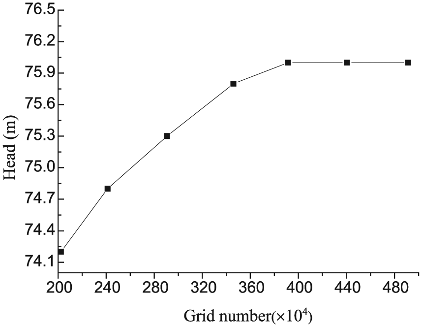
Variation curve of head with changes in grid number.

Figure 5.

Computational fluid mesh.

The material characteristic parameters of the rotor structure are listed in Table 1. In addition, the mesh of the rotor structure was generated in ANSYS Workbench 14.5, as shown in Figure 6.

Table 1.

Material parameters of impeller structure.

Density (kg/m³)	Young’s modulus (GPa)	Poisson’s ratio
7920	220	0.3

Figure 6.

Grids of rotor structure.

Coupled simulation setup

For the fluid calculation part, the 3D unsteady Reynolds-averaged Navier–Stokes equation solving uses ANSYS CFX 14.5 software. Turbulence model uses the SST k–ω model, and turbulence intensity is selected as 5%. The discretization in space is the high resolution of accuracy, and the second-order back Euler scheme is chosen for time discretization. The boundary conditions of inlet and outlet are as follows: inlet is set to total pressure of the static coordinate system and flow direction, and outlet uses mass flow rate outlet. Interface between suction and impeller and between impeller and diffuser is set to transient rotor stator. The mesh connection method is GGI. The solid surfaces are considered to no-slip wall boundary condition, and the standard wall function is used to calculate the boundary-layer variables. Also, wall roughness is set according to the actual situation. The roughness of the impeller walls is 0.0063 mm, and the roughness of the diffuser walls and the volute walls is 0.0125 mm. The coupling data use total forces and the fluid used was water; when the temperature is at 180°C and the pressure is below 27 bar, its density is 888.13 kg/m³, dynamic viscosity is 1.5065e−4 Pa·s, specific heat capacity is 4396.226 J·Kg⁻¹·K⁻¹, thermal conductivity is 0.67465 W·m⁻¹·K⁻¹, and the thermal expansivity is 7.4E−04K⁻¹. Time step is determined according to the angle of rotation of the impeller in each step. Impeller rotates 3° in each step. So, an impeller rotation cycle contains 120 time step. Total time includes 10 impeller rotation cycles. The average residual convergence criterion is set to be 1.0E−4.

Experimental validation

To validate the numerical results of the hydraulic performances of the RHRP, experimental data for the RHRP were carried out in the laboratory of the National Research Center of Pumps at Jiangsu University. The schematic diagram of an opened test rig is shown in Figure 7. A frequency inverter was used to adjust the speed of the motor during the starting and stopping period. Two pressure transmitters were mounted on the inlet and outlet pipes of the pump to measure static pressure. Then, the hydraulic head of the pump was calculated by these static pressure values. A relative pressure transmitter with a range of 0–4 bar was located on the inlet of the pump, and an absolute pressure transmitter with a range of 0–16 bar was located on the outlet of the pump. A turbine flow meter mounted on the downstream pipe was used to measure the flow rate. A flow control valve with motor was located at the downstream of the turbine flow meter in the pipeline. Its function is to adjust the flow rates during the test. Figure 8 shows the actual test rig.

Figure 7.

Schematic diagram of the test rig.

Figure 8.

Actual test rig.

The head is an important parameter to indicate the performances of the pump. The head of the RHRP was experimentally investigated in order to further verify the calculating results. According to the law of similarity, numerical simulation results were converted to test conditions. The curves of the head of RHRP obtained by both CFD and experimental methods are shown in Figure 9. It can be seen that the head predicted by numerical simulations does accord with the experimental results. The maximum deviation of the head between the CFD and the experiment data is below 4%.

Figure 9.

Hydraulic performance of RHRP.

Results and discussions

In this study, the RHRP performances were investigated under three required operating conditions which are Q = 120 m³/h (the lowest flow rate condition), Q = 910 m³/h (the design flow rate condition), and Q = 1475 m³/h (the maximum flow rate condition).

In addition to obtain the dynamic stress and displacement as a function of time, several monitoring points were defined on the rotor structure, as shown in Figure 10. P₀ was defined at bearing shaft shoulder. P₁ and P₂ were defined at the trailing edge of the blade near the shroud and the hub, respectively. P₃ was located on the wear ring of the impeller. The shaft, where the bearing was installed, was set to fixed support in transient structure dynamic analysis, as shown in Figure 10. In order to analyze the unsteady flow and the distribution of dynamic stress in RHRP, two coordinates were established, as shown in Figure 11. One was a stationary coordinate frame used for defining the impeller position marked as (x, y). The other rotating coordinate frame marked as (ξ, ψ) was used to define the circumferential position in the stationary coordinate frame. The positive y axis of the stationary coordinate frame spins a certain angle in anticlockwise direction and then overlaps the positive ψ axis of the rotating coordinate frame. This angle was defined to the rotating angle φ and used to resolve the rotation position of the impeller. In order to analyze the pressure fluctuation pattern on the outlet of the impeller, some monitoring points were located in the impeller’s outlet and each point be apart the rotating angle φ = 60°, as shown in Figure 11.

Figure 10.

Constraint of rotor and distribution of monitoring points on dynamic stress and displacement.

Figure 11.

Definition of coordinate systems and distribution of monitoring points on pressure fluctuation.

Figure 12 shows the streamline distribution at mid-span in the impeller and the diffuser under the three required conditions when φ = 0°, and the legend represents the velocity scale in the calculation domain. It can be seen that stable flow patterns are observed in the impeller and the diffuser, also the velocity is relatively low, when the flow is at the design flow. The velocity near the blade pressure side is larger than that near the blade suction side in the impeller, and a relatively low velocity appear near the blade pressure side of the impeller. When the flow reaches the maximum flow, there is an unstable flow in the diffuser, and vortex occurs in every diffuser vane. But when the flow decreases to the lowest operating flow, area of the vortex in the impeller passage and the diffuser vane is very large, also eddy becomes intensive, because the fluid constraint ability of the impeller is insufficient.

Figure 12.

Streamline distribution (m/s) at mid-span at different flow rates, φ = 0°: (a) Q = 120 m³/h, (b) Q = 910 m³/h, and (c) Q = 1475 m³/h.

The x and y components of the transient hydrodynamic force under different operating conditions are shown in Figure 12. And the time-average radial forces at different operating conditions in a impeller period are list in Table 2. The force magnitudes function as the rotation angle φ. A reference force of the forces is defined in equation (5). Furthermore, the normalized force magnitude F* is achieved based on equation (6)

F_{ref} = 0.5 ρ u_{2}^{2} b_{2} r_{2}

(5)

F^{*} = \frac{F}{F_{ref}}

(6)

where u₂ denotes the circumference velocity of the impeller tip, b₂ denotes the wide of impeller outlet, and r₂ denotes the radius of the impeller tip.

Table 2.

Time-average radial force at different operating conditions.

Average force	Flow rate (120 m³/h)	Flow rate (910 m³/h)	Flow rate (1475 m³/h)
x component (N)	−39.2	21.1	−40.9
y component (N)	−39.3	−33.8	−39.1

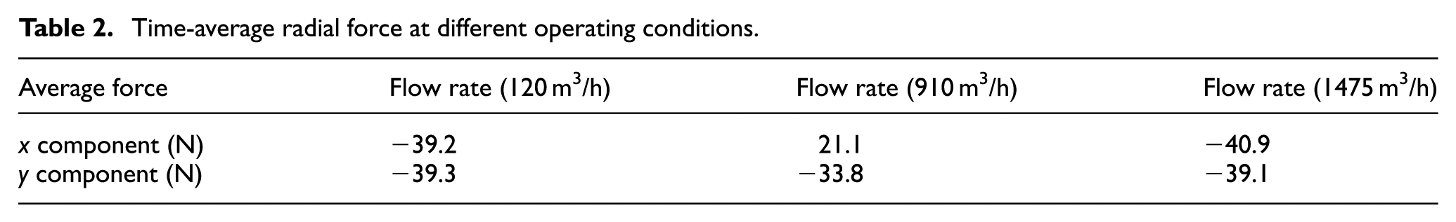
As shown in Table 2, the time-average radial force value is the smallest at the design condition. But the force values are almost equal when the RHRP operates under the lowest flow rate or the maximal flow rate. Figure 13 shows that the force magnitude at the maximum operating condition is the largest. Phase difference can be clearly seen among the results obtained under different conditions. The curves of the force y component have a different phase compared to the force x component.

Figure 13.

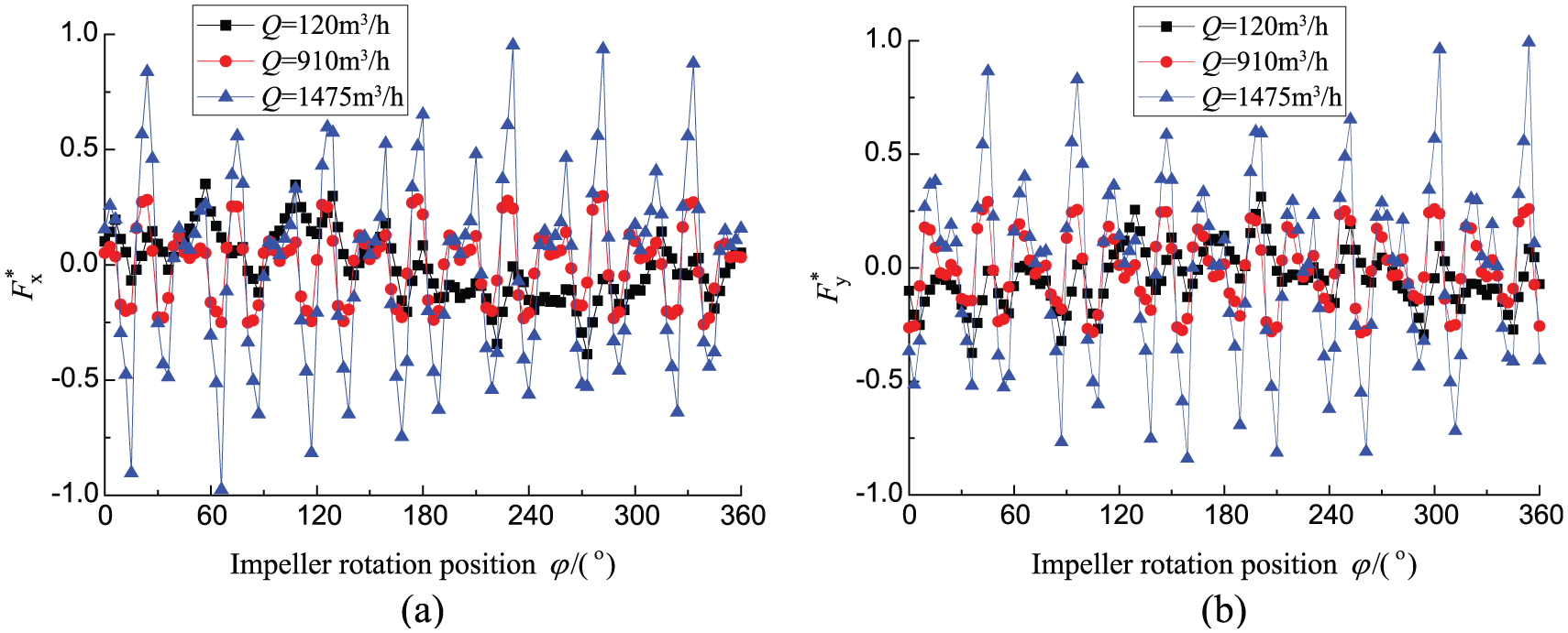
Transient hydrodynamic forces on the impeller blades: (a) force x component and (b) force y component.

To reveal the behaviors of the unsteady pressure, a non-dimensional pressure coefficient, C_p, is obtained using equation (7) in order to calculate the magnitude of the pressure fluctuations in a rotating cycle of the impeller

C_{p} = \frac{P - P_{ave}}{0.5 ρ u_{2}^{2}}

(7)

Figures 14 –16 show the frequency spectrum of pressure pulsation of the monitoring points P₄–P₉ under different conditions. It is clear that the domain frequencies of pressure fluctuations of the monitors are 5, 10, 15, and 20 f_n (rotating shaft frequency) under different operating conditions. Also, compared to other monitoring points, the monitoring point P₇ has relatively large peak values for the lowest flow condition and the design flow condition, the frequency of which is 5 f_n. According to Figure 23, the relatively large peak value for the maximum flow condition is obtained on P₆, the frequency of which is 15 f_n. The results of comparison are obtained on all monitoring points, and it can be seen that the magnitude of the relatively large peak for the design condition is the lowest.

Figure 14.

Frequency spectrum of pressure pulsation of monitoring points under the flow rate Q = 120 m³/h.

Figure 15.

Frequency spectrum of pressure pulsation of monitoring points under the flow rate Q = 910 m³/h.

Figure 16.

Frequency spectrum of pressure pulsation of monitoring points under the flow rate Q = 1475 m³/h.

The dynamic stress in the rotor structure is calculated based on the fourth strength theory. Since the sheer stress is much smaller than the normal stress in this case, the von Mises or equivalent stress is calculated as follows

σ_{eq} = \sqrt{\frac{1}{2} [{(σ_{x} - σ_{y})}^{2} + {(σ_{y} - σ_{z})}^{2} + {(σ_{z} - σ_{x})}^{2}]}

(8)

Figure 17 shows the time-dependent maximum equivalent stress on the monitoring point P₀ in which the results are calculated using FSI method combined with the structure response analysis under different conditions. There is very obvious fluctuation for all flow rate conditions. It can be seen that the curves have a same phase. And there are four peak values and trough values in an impeller rotating cycle at different flow rate conditions, and the adjacent peak or valley values apart 90° are clearly observed. The equivalent stress values increase with the flow rates because the shaft power also becomes larger with the increase in the flow rate. The equivalent stress values are between 250 and 286 MPa under the lowest flow rate condition, between 276 and 310 MPa at the design flow rate condition, and between 304 and 344 MPa under the maximum flow rate condition. Compared to Figures 18 and 19, the relatively large equivalent stress value of P₀ is so much higher than that of P₁ and P₂. So, when RHRP operates in nuclear power plants, fatigue damage is most likely to occur on the shaft near where the loose bearing is installed.

Figure 17.

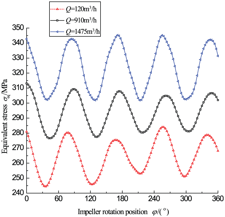
Time-variant equivalent stress distribution on P₀ for different operating conditions.

Figure 18.

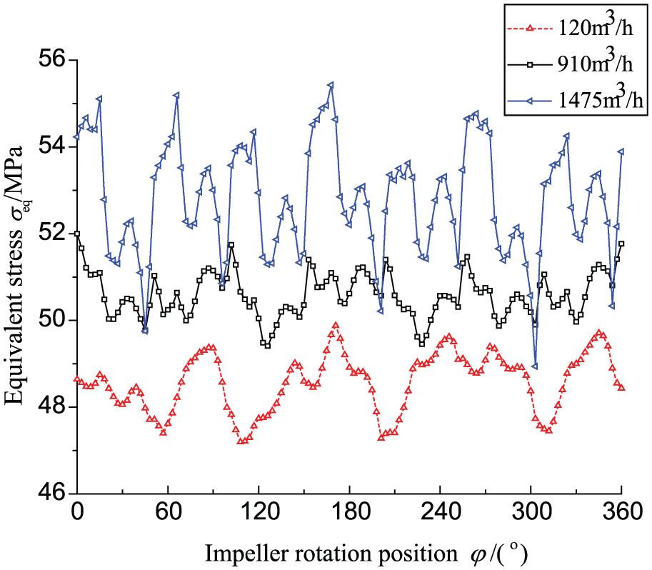
Time-variant equivalent stress distribution on P₁ for different operating conditions.

Figure 19.

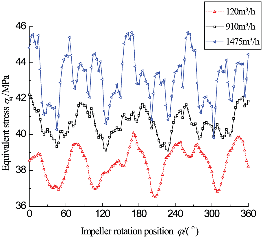
Time-variant equivalent stress distribution on P₂ for different operating conditions.

The equivalent stress on the monitoring points P₁ and P₂ is presented as the function of the impeller’s rotation angle φ, as shown in Figures 19 and 20. Their curves show obvious fluctuation and specific phase differences. The relatively large equivalent stress values of P₁ and P₂ increase with increasing flow rates. The equivalent stress values of the monitoring point P₁ vary from 48.5 to 55.5 MPa at the largest flow rate condition and that of wave from 47 to 50.3 MPa under the lowest flow condition. Moreover, at the rated flow condition, the equivalent stress values of the monitoring point P₁ fluctuate from 49.7 to 52 MPa, which is smaller than other conditions. The pressure fluctuation value at the impeller’s outlet under the rated flow condition is lower than the other conditions. Compared to the equivalent stress values of the monitoring point P₂ shown in Figure 2, the relatively large and relatively small equivalent stress values of P₁ are much higher among all conditions.

Figure 20.

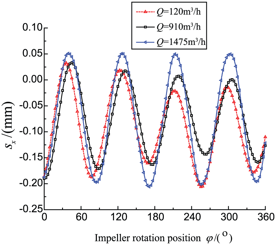
Displacement at P₃ in x direction.

The comparisons of the displacement at the monitoring points P₁ and P₃ numerical results considering strong FSI under different conditions are shown in Figures 20 –23. The curves of the displacement track on monitoring points in two directions are obtained. The curves of the displacement are the function of the impeller’s rotation angle φ for one rotating cycle of the impeller. Both the amplitude of the displacement and the phase of the displacement were investigated.

Figure 21.

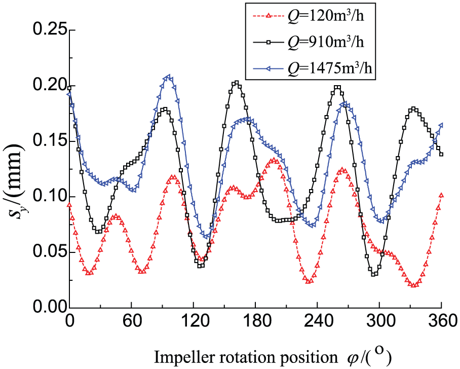
Displacement at P₃ in y direction.

Figure 22.

Displacement at P₁ in x direction.

Figure 23.

Displacement at P₁ in y direction.

According to Figure 20, the curves of the displacement at P₃ in x direction with four peak values and valley values in an impeller rotating cycle are distinctly observed, and the adjacent peak or valley values apart 90° are clearly observed. It can be seen that the magnitude of the displacement at the maximum flow condition is the largest. Furthermore, the displacement values between −0.22 and 0.51 mm are obtained. The y-component curves of displacements at the monitoring point P₃ for different conditions are shown in Figure 21. Phase differences can be clearly seen among the results captured at all different conditions. The largest value of the smallest flow rate condition exhibits at the impeller’s rotation angle φ = 210°, and that of the rated operating condition and the largest flow rate condition display at the impeller’s rotation angle φ = 165° and φ = 100°, respectively. The y-direction displacement values are between 0.02 and 0.13 mm, 0.03 and 0.22 mm, and 0.51 and 0.23 mm at the lowest; the design and the maximum flow condition are obtained, respectively.

Compared to the x-direction displacement curves of the monitoring point P₃, the curves of the monitoring point P₁ exhibit similar variation tendency. But the magnitude of the monitoring point P₁ is larger. It can be seen that the x-direction displacement values at the lowest flow rate condition are between −0.55 and 0.54, under the design flow rate condition between −0.23 and 0.74 mm, and for the maximum flow rate condition between −0.38 and 0.79 mm. It is clear from Figure 17 that the curves of the y-direction displacement of the monitoring point P₁ at different conditions have different phases obviously. The y-direction displacement values of the monitoring point P₁ are between 0.73 and 0.99 mm, 0.83 and 1.21 mm, and 0.87 and 1.22 mm at the lowest; the design and the maximum flow condition are obtained, respectively.

It is clear that the displacement values of the monitoring point P₃ in x direction or y direction are lower than wear ring clearance (0.4 mm). So, a wear ring clearance value of 0.4 mm is suitable for this RHRP. The relatively large displacement value of P₁ is higher than P₃ because the flow pressure at the impeller’s outlet is larger than that of the impeller’s inlet.

Conclusion

The internal flow in RHRPs is simulated using Reynolds-averaged Navier–Stokes equations with the SST k–ω turbulence model, and the dynamic stress and displacement of the rotor are calculated using transient structure dynamic analysis combined with the FSI strategy. The transient hydrodynamic forces on the impeller, the stress and displacement distribution in the rotor, and the pressure fluctuation of the impeller’s outlet are investigated. The following conclusions are made:

The radial force value at the design flow rate condition is the smallest. The force magnitude is the largest under the maximum flow rate operating condition.

The relatively large displacement value of the impeller’s outlet is higher than that of the wear ring of the impeller due to the transient force caused by the flow pressure fluctuation at the impeller’s outlet, which is stronger than that of the impeller’s inlet. Moreover, both in x and y directions, the displacement values of the wear ring of the impeller are lower than the wear ring clearance.

The equivalent stress value of the shaft, near where the loose bearing in rotor is installed, is much higher than that of other place under all flow rate conditions. Also, the equivalent stress on the trailing edge near the shroud is larger than that on other part of blades.

The domain frequencies of pressure fluctuations of the monitoring points at the impeller’s outlet are 5, 10, 15, and 20 f_n (rotating shaft frequency). The frequency of the relatively large peak value of some monitoring points for the maximum flow condition is bigger than those for the other two conditions. And, the frequency of the relatively large pressure fluctuations of the monitoring points located at different positions is different.

Footnotes

Appendix 1

Academic Editor: Yuning Zhang

Declaration of conflicting interests

The author(s) declared no potential conflicts of interest with respect to the research, authorship, and/or publication of this article.

Funding

The author(s) disclosed receipt of the following financial support for the research, authorship, and/or publication of this article: This study was supported by the Foundation Research Project of Jiangsu Province (The Natural Science Fund no. BK20160539), a project funded by the Priority Academic Program Development of Jiangsu Higher Education Institutions, Jiangsu University Senior Personnel Scientific Research Foundation (no. 15JDG073), and the Scientific Innovation Program in Colleges and Universities of Jiangsu Province (no. KYLX15_1065).

References

Zhang

Guo

Wang

WQ.

FEM simulation of turbulent flow in a turbine blade passage with dynamical fluid-structure interaction. Int J Numer Meth Fl 2009; 61: 1299–1330.

Zhang

Guo

Wang

WQ.

Large eddy simulation of turbulent flow in a true 3D Francis hydro turbine passage with dynamical fluid-structure interaction. Int J Numer Meth Fl 2007; 54: 517–541.

Muench

Ausoni

Braun

. Fluid-structure coupling for an oscillating hydrofoil. J Fluids Struct 2010; 26: 1018–1033.

Campbell

Paterson

EG.

Fluid-structure interaction analysis of flexible turbomachinery. J Fluid Struct 2011; 27: 1376–1391.

Xiao

Zhu

Yang Wei

. Stress analysis of Francis hydraulic turbine runner based on FSI. J Drain Irrig Mach Eng 2013; 31: 862–866 (in Chinese).

Jiang

Yoshimura

Imai

. Quantitative e-valuation of flow-induced structural vibration and noise in turbomachinery by full-scale weakly coupled simulation. J Fluid Struct 2007; 23: 531–544.

Zienkiewicz

Taylor

RL.

The finite element method. Oxford: Butterworth-Heinemann, 2000.

Tai

Bals

Zhao

. An efficient parallel computation of unsteady incompressible viscous flow with elastic moving and compliant boundaries on unstructured grids. Int J Numer Meth Eng 2005; 64: 2072–2104.

Tai

Zhao

Liew

KM.

Parallel-multigrid computation of unsteady incompressible viscous flows using a matrix-free implicit method and high-resolution characteristics-based scheme. Comput Method Appl M 2005; 194: 3949–3983.

10.

Eladi

Chatterjee

Gupta

AD.

An efficient numerical method for predicting the performance of valveless micropump. Smart Mater Struct 2012; 21: 115012 (12 pp.).

11.

Pei

Yuan

JP.

Fluid-structure coupling effects on periodically transient flow of a single-blade sewage centrifugal pump. J Mech Sci Technol 2013; 27: 2015–2023.

12.

Jiang

Zhai

Wang

LQ.

Fluid-structure interaction analysis of annular seals and rotor systems in multi-stage pumps. J Mech Sci Technol 2013; 27: 1893–1902.

13.

Yuan

Pei

Yuan

JP.

Numerical investigation on fluid structure interaction considering rotor deformation for a centrifugal pump. Chin J Mech Eng 2011; 24: 539–545.

14.

Pei

Benra

Dohmen

HJ.

Application of different strategies of partitioned fluid-structure interaction simulation for a single-blade pump impeller. Proc IMechE, Part E: J Process Mechanical Engineering 2012; 226: 297–308.

15.

Pei

Dohmen

Yuan

. Investigation of unsteady flow-induced impeller oscillations of a single-blade pump under off-design conditions. J Fluid Struct 2012; 35: 89–104.

16.

Pei

Yuan

JP.

Dynamic stress analysis of sewage centrifugal pump impeller based on two-way coupling method. Chin J Mech Eng 2014; 27: 369–375.

17.

Benra

F-K

Dohmen

Wan

. (2006, January). Determination of pump impeller deflections: comparison of FSI-simulations to measurements. In: Proceedings of the ASME 2006 2nd Joint US-European Fluids Engineering Summer Meeting Collocated With the 14th International Conference on Nuclear Engineering, January 2006, pp.291–296. ASME.

18.

Langthiem

MA.

A numerical study of flow-induced noise in a two-dimensional centrifugal pump. Part I: hydrodynamics. J Fluids Struct 2004; 19: 349–368.

19.

Kato

Yamade

Wang

. Prediction of the noise from a multi-stage centrifugal pump. In: ASME fluids engineering division summer meeting, Houston, TX, 19–23 June 2005, Part B, pp.1273–1280. New York: ASME.

20.

Yuan

Zhu

Zhou

. Pressure fluctuation in residual heat removal pumps. J Drain Irrig Mach Eng 2015; 33: 475–480.

21.

Lei

Shan

Liang

. Numerical simulation of unsteady cavitation flow in a centrifugal pump at off-design conditions. Proc IMechE, Part C: J Mechanical Engineering Science 2014; 228: 1994–2006.

22.

Tan

Zhu

Wang

. Numerical study on characteristics of unsteady flow in a centrifugal pump volute at partial load condition. Eng Computation 2015; 32: 1549–1566.

Investigation of dynamic stress of rotor in residual heat removal pumps based on fluid–structure interaction

Abstract

Keywords

Introduction

FSI simulation and experimental validation

FSI method

Mesh generation and mesh independence check

Coupled simulation setup

Experimental validation

Results and discussions

Conclusion

Footnotes

Appendix 1

Declaration of conflicting interests

Funding

References