Sage Journals: Discover world-class research

Abstract

Health condition monitoring for rotating machinery has been developed for many years due to its potential to reduce the cost of the maintenance operations and increase availability. Covering aspects include sensors, signal processing, health assessment and decision-making. This article focuses on prognostics based on physics-based models. While the majority of the research in health condition monitoring focuses on data-driven techniques, physics-based techniques are particularly important if accuracy is a critical factor and testing is restricted. Moreover, the benefits of both approaches can be combined when data-driven and physics-based techniques are integrated. This article reviews the concept of physics-based models for prognostics. An overview of common failure modes of rotating machinery is provided along with the most relevant degradation mechanisms. The models available to represent these degradation mechanisms and their application for prognostics are discussed. Models that have not been applied to health condition monitoring, for example, wear due to metal–metal contact in hydrodynamic bearings, are also included due to its potential for health condition monitoring. The main contribution of this article is the identification of potential physics-based models for prognostics in rotating machinery.

Keywords

Bearings condition monitoring creep damage mechanics failure fracture mechanics gears modelling rotating machinery

Introduction

Prognostics and Health Management (PHM) refers to the capability to assess the current (diagnostics) and future (prognostics) health state of a system, which can be a machine, a process or a vehicle. As a result, the maintenance plan can be optimized depending on the current health status of the system called predictive maintenance or condition-based maintenance (CBM), instead of relying on historical data and life estimation calculations (preventive maintenance) or reacting only when a failure occurs (reactive maintenance).¹

The main benefits of a CBM strategy are the time and cost reduction due to the higher efficiency of planned maintenance and the optimization of the component life compared to preventive strategies.² However, these benefits must overcome the additional cost of the technology required to implement CBM. Additional benefits include the reduced mean maintenance time due to fault localization, the reduced disruption and the increased safety due to the reduction of unexpected failures.^3,4

The information generated by a PHM system can be divided into diagnostics and prognostics: diagnostics includes anomaly detection, fault isolation, fault classification and its uncertainty;⁵ while prognostics include the estimation of the remaining useful life (RUL), the uncertainty of the prediction and incipient fault detection. Also diagnostics and prognostics knowledge can be used for future improvements of the design.^6,7

In order to evaluate the health of a system, the various techniques are commonly categorized into data-driven models (DDMs), physics-based models (PbMs) and hybrid models.^8–10 DDMs are based on statistical- and machine-learning techniques and do not rely on the knowledge of the physics that govern the system or its degradation mechanisms:⁹ these techniques have proven successful for fault detection,¹¹ classification¹² and RUL estimation.¹³ PbMs consist in the use of mathematical models that describe the physics of the component to assess its current and future health. The performance of PbMs depends on the capability of the models to accurately represent the failure and degradation phenomena. Hybrid models refer to the integration of different models, either using various approaches depending on the task, for instance a DDM for diagnostics and a PbM for prognostics,^14–18 or a combination of several models that represent the same phenomena to obtain a more robust health assessment, so-called ensemble models.^19,20

The main advantages of machine-learning techniques are their potential to be used in several systems as knowledge of the physics of the system is not required, thus being easily scalable to different systems. However, there are problems such as risk of over fitting¹⁶ and the necessity of large training data sets compared to PbM approaches.⁹ Additionally, the synergies between PbMs and models used during the design phase make them particularly suitable when the health condition monitoring system is being developed during the design phase.¹⁰ However, PbMs are not easily scalable because they are system specific and it can be challenging to obtain measurable indicators directly related to the outputs of the PbM.⁵

Reviews covering the state of the art of health condition monitoring for rotating machinery have already been published focusing on the methodologies and algorithms of PHM in rotating equipment,^9,21 and specific techniques such as the empirical mode decomposition for fault diagnosis²² and vibration analysis.²³ However, the state of the art of PbM for rotating machinery has not been reviewed in depth; papers focused on PHM for rotating machinery normally include a section mentioning significant PbM approaches, but the description of the principles behind those models is limited. This article describes the principles behind the most relevant PbM for rotating machinery and the factors that have to be taken into account when selecting a model for PHM are discussed.

The aim of this article is to review the state of the art of prognostics for rotating machinery based on PbMs. The most important failure modes and the models available to represent their degradation mechanisms are identified, including not only the models already applied on PHM for rotating machinery, but also models that can potentially be used in the future. The concept of PbM and a brief review of parameter estimators are presented in the PbM approach section. Failure modes of rotating machinery section include common failure modes of rotating machinery and examples of PHM solutions for them. The well-accepted models of degradation mechanisms of rotating machinery are described in the relevant degradation models section. Finally, the section ‘Conclusion’ summarizes the findings of the article and discusses the challenges of applying PbMs for diagnostics and prognostics of rotating machinery.

PbM approach

PbM approaches, also referred to as model-based approaches, assess the health of the system by solving a set of equations derived from engineering and science knowledge,⁵ either for diagnostics or for prognostics. However, the main advantage of PbMs consists of using degradation models to predict long-term behaviour.²⁴ A generic process to develop prognostics based on PbMs that consider a set of equations that define the dynamics and the degradation of the system was proposed by Luo et al.²⁵ and is shown in Figure 1. It consists of a model of the system and its degradation, where fast dynamic variables represent the behaviour of the system, and slow dynamic variables determine degradation of the system, where random scenarios are simulated and compared to measurable data to identify the appropriate scenario (feature estimation) and estimate the RUL.

Figure 1.

Physics-based approach.²⁵

Normally, for diagnostics, a fault is detected by comparison between the outputs of the PbM and the measurements from the real system. An example of diagnostics using PbMs is the classification of bearing defects by measuring the natural frequencies of the components of the bearing, obtained from knowledge of the physics of the system, and deviations from normal values are used as health indicators as shown by Li et al.²⁶

It should be noted that to develop prognostics capabilities, prior knowledge of the current health status of the system (diagnostics) is required. For prognostics based on PbMs, degradation models are used to represent the degradation mechanisms of the system and the RUL can be estimated as an output of these models. For instance, degradation models based on Paris law²⁷ to represent crack growth have been used by several authors to estimate the RUL of systems subject to fatigue.^14,28–33

Health condition monitoring algorithms are normally classified into PbMs and DDMs, but the benefits of both approaches can be combined to obtain more robust algorithms called hybrid models. Orsagh et al.³⁴ proposed a generic framework (Figure 2) that used DDMs for diagnostics and a PbM for prognostics of bearings spalling by combining sensor data for diagnostics with model-based and historical data for prognostics. A similar approach is proposed by Zio and Di Maio,¹⁴ who applied Paris law for crack growth estimation (prognostics) and a relevance vector machine method for fault detection (diagnostics), while Pantelelis et al.¹⁵ were able to detect faults in a naval turbocharger combining finite element models of the system and an artificial neural network (ANN) for fault identification using vibration analysis.

Figure 2.

Hybrid model.³⁴

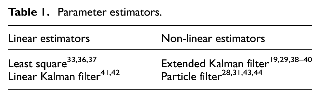
For prognostics, regardless of the approach (PbM, DDM or hybrid), the health condition monitoring algorithm will provide an assessment of the current health of the system, normally by measuring a health indicator, and a prediction of the future health of the system. That prediction should be as accurate as possible, but there are always errors between the predicted value of a health indicator and the measured one. Thus, it is important to have the capability to adjust the model in order to minimize these differences based on the past errors between the predicted health indicator and the measured ones. PbMs can be combined with parameter estimators to minimize these errors in real time.² A unified formulation has been proposed by Jaw and Wang³⁵ to implement parameter estimators into PbMs given a generic set of system equations. The most common parameter estimators are shown in Table 1. Linear estimators are less computationally expensive, but if the system behaviour is clearly more sophisticated non-linear algorithms are needed.

Table 1.

Parameter estimators.

Linear estimators	Non-linear estimators
Least square^33,36,37	Extended Kalman filter^{19,29,38–40}
Linear Kalman filter^41,42	Particle filter^28,31,43,44

Failure modes of rotating machinery

The development of PbMs requires an understanding of the system during normal operation and when a failure occurs. A failure is considered when a function of the system cannot be executed. It should be noted that ‘failure mode’ refers to the description of how a function of the system is no longer fulfilled, and a ‘degradation mechanism’ refers to the process that leads to a failure.⁴⁵

The main contribution of this article is the review of potential degradation models that can be used for health condition monitoring. Those degradation mechanisms represent the phenomena behind a specific failure mode. This section describes relevant failure modes and their degradation mechanisms. A comprehensive review of those degradation mechanisms is given in the following section.

The most common failure modes of typical components of rotating machinery are analysed and current health condition monitoring algorithms are discussed; these algorithms are summarized in Table 2. Three typical components of rotating machinery are considered:

Gears;

Rolling bearings;

Hydrodynamic bearings.

Table 2.

Health condition monitoring algorithms classified by component and failure mode.

Gears	Bearings
Scuffing⁴⁶	Fatigue: spalling/pitting^{34,36,37,47–59}
Pitting^60–64	Localized defects^65–69
Crack detection^70,71	Wear^72–74
Crack length estimation^32,75–77	Damage location^26,78–82
Tooth breakage^11,62,83	Geometrical imperfections^26,55
	Contaminants⁸⁴
	Metal–metal contact^85,86

Gears

Gears are subjected to high cyclic loads and harsh environments, thus being able to monitor the health of the gears is of major importance. In this review, the failure modes of gears are classified following the guidelines of the ISO 10825:1995,⁸⁷ which classifies gear failures as shown in Figure 3. Each failure mode will be described and their corresponding PHM solutions will be briefly reviewed.

Figure 3.

Gear damage terminology.

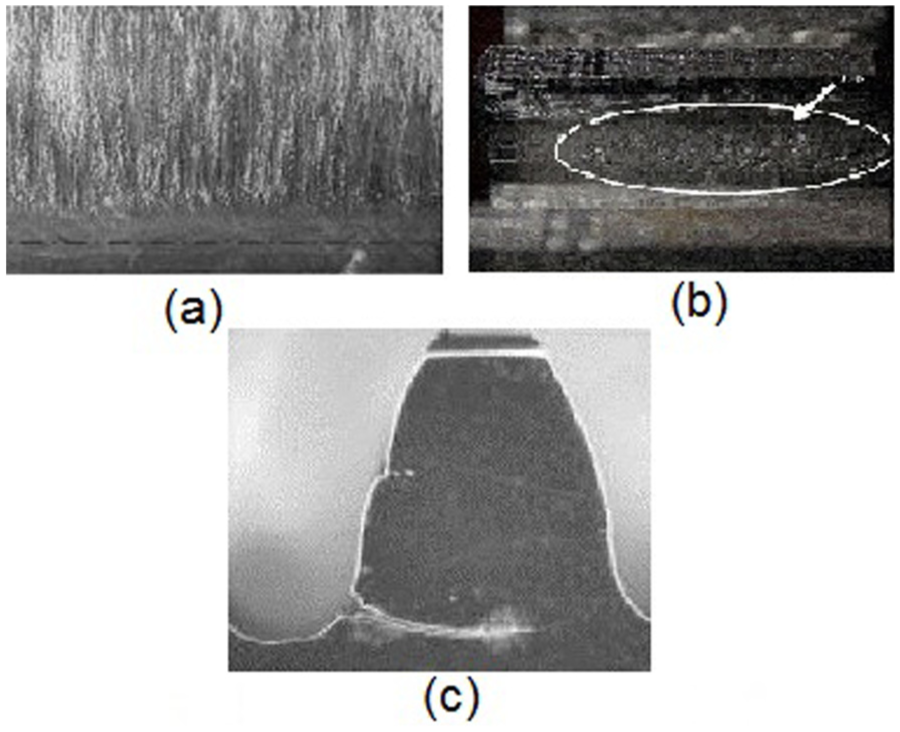
Scuffing (Figure 4(a)) consists in damage in the sliding direction due to metal–metal contact caused by insufficient lubrication, causing the subsequent transfer of material and increased vibrations and noise. Castro and Seabra⁴⁶ proposed a simplified model that does not consider surface parameters and a more sophisticated mixed lubrication model that required roughness parameters to detect scuffing in gears under a variety of speeds, torques and oil bath temperatures. Therefore, scuffing can be modelled using wear models, in particular models that predict metal–metal contact between the teeth.

Figure 4.

Gear defects: (a) scuffing,⁴⁶ (b) pitting⁶⁰ and (c) crack.³²

Permanent deformations include indentation and scratches that can be caused by foreign objects, or permanent deformation of the teeth. Permanent deformation consists of plastic deformation, which occurs under excessively high stresses; thus, excessive load can cause permanent deformations; the accumulated plastic deformation mechanism consists of low cycle fatigue (LCF).

The cyclic stresses produced in gears also cause high cycle fatigue (HCF), characterized by removal of material. This type of damage can be divided into pitting and spalling. Pitting consists of surface fatigue between rolling and sliding contacts, leading to small scattered holes as shown in Figure 4(b). If initial pitting is not detected, it can lead to spalling, which consists of macro-pitting caused by the association of small cracks into bigger ones.⁸⁷ The degradation mechanisms and the differences between pitting and spalling have been discussed in depth by Ding and Rieger.⁸⁸ Pitting and spalling are caused by stresses that do not lead to permanent plastic deformations; instead, the main degradation mechanism is driven by the high number of cycles for a relatively low load. This degradation mechanism is HCF.

Cracks (Figure 4(c)) are caused by defects in the gear due to deficient material properties, the manufacturing process or fatigue.⁸⁷ Crack detection has caught the attention of several authors and promising results have been obtained not only for diagnostics, but also for prognostics through the estimation of the crack length and its correlation with the RUL.

For diagnostics, simple DDMs as statistical parameters can be used as health status features. For instance, Zakrajsek and Lewicki⁷⁰ detected spur gear tooth cracks before complete fracture occurred using several statistical estimators. For prognostics of cracks, Feng et al.⁷⁵ used spectrum features to detect a crack and predict its evolution. However, the results were only based on simulations. A more common approach for prognostics consists of a PbM based on Paris law²⁷ to model the degradation mechanism and estimate the crack growth rate, which is an indicator of the RUL. Kacprzynski et al.⁷⁶ proposed the combination of Paris law along with a simplified two-dimensional (2D) finite element analysis (FEA) for RUL estimation. This approach was extended by Li and Lee,³² who developed a dynamic model of a transmission to estimate the loads, a FEA to infer the stresses and an algorithm based on Paris law to obtain the RUL. The same approach was later used by Kacprzynski et al.⁷⁷ for prognostics of H-60 helicopter gear cracks using a more sophisticated three-dimensional (3D) FEA to estimate the loads, including crack initiation and crack propagation PbMs. Therefore, it is evident that the most suitable degradation models consist of representing crack growth.

Tooth breakage, total or partial, can have diverse causes and be produced by a single very high load or after a few cycles of high loads and the fracture can vary from ductile to brittle fracture.⁸⁷ Using vibration analysis, Wu et al.⁸³ differentiated between broken, worn or healthy teeth applying the support vector machine (SVM) technique. Partial breakage of the tooth, called chipping, can also be detected by looking at the differences in the mesh frequency side bands in the time–frequency domain.^11,62 This failure mode is caused by a single event; there is no continuous degradation from healthy to faulty conditions.

Bearings

Rolling bearings

Bearings are necessary to provide support for the rotating machinery, transmitting the axial and radial loads from the rotating component to the structure, and to minimize the friction losses in the sliding direction. This section will analyse rolling bearings, and hydrodynamic bearings will be covered in the next subsection. The failure modes are normally classified depending on the components that are damaged, differentiating between inner race, outer race, rolling elements and cage failures.^26,79,80

The failure modes of rolling bearings can also be divided into failures caused by excessive operational conditions, by the lubricant and by assembly and disassembly errors⁸⁹ as shown in Figure 5.

Figure 5.

Damage causes in rolling bearings.

Being able to detect lubrication anomalies, which are responsible of 50% of all the premature bearing failures in oil-lubricated bearings⁹⁰, would help to detect incipient failures by controlling the cause of the damage instead of the effect. Iyer et al.⁹¹ reviewed the techniques available to detect lack of lubrication and contamination and stated that even if ferrous debris sensors and oil condition monitoring can provide very valuable information, they cannot be applied to oil bath lubricated bearings.

Most of the research has been focused on detecting defects through vibration analysis and acoustic emission (AE). El-Thalji and Jantunen⁹² stated that bearing faults are assumed to produce impulses that affect the vibration spectrum and conducted an extensive review of the state of the art of PHM of rolling bearings covering bearing faults, monitoring techniques and signal processing methods. Previous reviews of health monitoring of rolling bearings can also be found.^93–96

Sunnersjö⁵⁵ studied the changes in the vibration response of rolling bearings subjected to geometrical imperfections, spalling and abrasive wear using time-history diagrams, spectrograms and time–frequency analysis. Spalling also was studied by Sawalhi and Randall⁵⁶ using vibration analysis and time–frequency analysis to take into account the low-frequency spectrum of the incipient spalling and the high-frequency impulsive response of severe spalling. The effect of contaminants in the vibration response of rolling bearings is analysed by Maru et al.,⁸⁴ who found significant differences in root mean square (RMS) values for frequencies between 600 and 10,000 Hz and compare the effect of contaminants using different particle sizes.

AE techniques have also proven to be effective in detecting defects in lubricated sliding contacts, including rolling and hydrodynamic bearings. Boness and McBride⁷⁴ found an empirical relationship between AE, RMS and wear volume removed. An effect caused by adhesive and abrasive degradation mechanisms in lubricated point contacts. Price et al.⁵⁸ used AE and vibration analysis in the time and frequency domain showing the potential of AE to detect incipient pitting with a high signal-to-noise (S-N) ratio. Guo and Schwach⁵⁹ studied the effectiveness of AE parameters to detect rolling contact fatigue in point contacts, finding that RMS and amplitude were the better indicators of surface defects. Rahman et al.⁵⁰ were able to detect and localize incipient fatigue damage in rolling contacts using the AE hit count rate. Choudhury and Tandon⁶⁶ detected incipient inner race and roller bearing faults by measuring AE counts. He et al.⁶⁷ applied a more sophisticated technique, the wavelet scalogram in the time–frequency domain, to detect defects in rolling element bearings using AE under different operational conditions.

AE has also proven effective in detecting micro-cracks in the surfaces of axial bearings earlier than with vibration analysis by looking at the hit count rate and the amplitude of the signal.^51,52 Elforjani and Mba⁵³ also detected and located fatigue damage in axial bearings using AE. Jamaludin and Mba^68,69 proved that AE is a powerful technique to detect damage of rolling bearings at extremely low speeds.

Less common techniques have also been used and compared to vibration and AE analysis. For instance, Kim et al.⁶⁵ compared vibration analysis with ultrasounds using statistical parameters in the time domain and spectral analysis to detect damage in rolling bearings and obtained better results using ultrasounds for low bearing speeds. Sun et al.⁷² compared AE and an electrostatic wear monitoring method that measures the electrical charge in the bearing and correlated it with the wear degradation finding that both techniques are able to detect wear caused by metal–metal contact. Harvey et al.⁷³ also validated an electrostatic wear detection method for rolling contacts able to detect seeded faults prior the total failure occurred.

Regarding the health condition monitoring algorithms, machine learning also proved to be a useful approach commonly used for fault classification. Paya et al.⁷⁸ obtained features from the wavelet transform, later used for training and testing an ANN capable of differentiating between bearing faults in the inner race of the bearing and faults in the adjacent gears; while Jack and Nandi⁸⁰ compared bearing features from time and frequency domains by combining an ANN and a SVM algorithm to detect inner race, outer race, ball and cage faults. Li et al.²⁶ used the frequency domain of the vibration signal from rolling bearings to detect ball and inner race damage along with looseness using the fundamental bearing frequencies as features to train an ANN. Tang et al.⁷⁹ also detected cracks in bearings and classified them as ball, inner race or outer race crack with 92% accuracy in a wind turbine transmission using a SVM algorithm. Du et al.⁸¹ also differentiated between ball, inner and outer race failures using a modified SVM algorithm with 94% accuracy.

Health condition monitoring algorithms based on PbMs are not too many when compared to DDMs. However, there are important examples of PbMs for rolling bearings. McFadden and Toozhy⁴⁷ detected spalling using a PbM that calculates the characteristic frequency of damage caused by spalling and synchronously averaged the frequency response with the rotating speed of the shaft and was able to detect spalling and estimate the distribution of the damage in the inner race. Zong et al.⁹⁷ developed a PbM to identify spalling in the inner rig using a FEA model of the defect and its vibration response. Another important PbM for prognostics of rolling bearings was introduced by Li et al.,³⁷ who were able to estimate the RUL as a function of the size of the spalls using a deterministic degradation model similar to Paris law, further improved to include the stochastic of the failure.³⁶ Orsagh et al.³⁴ later applied a similar approach to detect spalling and estimate the RUL in rolling bearing. Qiu et al.⁴⁸ proposed a different PbM approach to detect damage in bearings, consisting in a dynamic model of the bearing that correlates the natural frequencies and their amplitude, obtained from the vibration response, with the stiffness of the system. This approach is later integrated with a degradation model that defines the damage as a function of the stiffness and can be used to estimate the RUL of the bearing. However, Sun et al.⁸² argue that methods based on characteristic frequencies are not accurate enough and proposes a DDM based on fuzzy logic to classify outer race, inner race and ball bearing faults with 94.7% accuracy.

Different rolling failure modes have been analysed. Some failure modes, such as contaminants and geometrical imperfections, are caused by external factors and degradation mechanisms cannot be modelled, because the particle size or composition of contaminants and the dimensions of the geometrical imperfections are unknown. Fault isolation techniques to differentiate between inner/outer or ball failures lead to wear of the faulty sub-component; the fundamental frequencies of the components can be modelled and monitored to localize the failure. In order to track spalling and pitting in rolling bearings, as it occurs with gears, the degradation mechanism consist of fatigue due to excessive cycles and loading. HCF models and spalling growth models, similar to Paris law can be used.

Hydrodynamic bearings

The function of hydrodynamic bearings and rolling bearings is identical: to provide low friction in the sliding direction and to transmit the radial and axial loads. The main difference is the type of contact, in which both surfaces slide without any intermediate component.

The most typical failure modes of hydrodynamic bearings⁹⁸ are shown in Table 3. Zeidan and Herbage⁹⁹ also reached the same conclusions after analysing the most common failures of hydrodynamic bearings.

Table 3.

Major causes of premature hydrodynamic bearing failure.

Major causes of premature bearing failure
Dirt	45.4%
Incorrect assembly	12.8%
Misalignment	12.6%
Insufficient lubrication	11.4%
Overloading	8.1%
Corrosion	3.7%
Improper journal finish	3.2%
Other	2.8%

Dirt, incorrect assembly and defects in the manufacturing process are particularly difficult to monitor. Thus, most of the research has been focused on detecting insufficient lubrication, which is directly related to metal–metal contact and leads to rapid degradation. The main failure mechanism related to insufficient lubrication is scuffing, already discussed for gears, which eventually develops into seizure.¹⁰⁰ Tanaka¹⁰¹ demonstrates experimentally the effect of flow rate and speed in the lubrication phenomena by measuring eccentricity and cavitation under insufficient lubrication compared to fully flooded lubrication. Even if a film of lubricant remains and there is not metal–metal contact, fatigue damage can occur due to the cyclic stresses on the surface of the bearing as shown by Huang et al.,¹⁰² who studied fatigue wear in hydrodynamic bearings.

A variety of failure analysis of hydrodynamic bearings can be found in the literature. Vencl and Rac¹⁰³ studied the failures of over 180 engine bearings, finding that abrasive wear is the predominant degradation mechanism, followed by adhesive and fatigue wear, as shown in Figure 6. They also identified the causes corresponding to each degradation mechanism:

Contaminants in the lubricant: provoke abrasive wear;

Overload: provokes fatigue wear caused by excessive stresses on the surfaces of the bearing;

Insufficient clearance: provokes adhesive wear;

Insufficient lubrication: provokes adhesive wear;

Metal–metal contact: provokes adhesive wear.

Figure 6.

Percentage occurrence of types of hydrodynamic bearing damage.¹⁰³

A comparison between temperature measurements, electric resistance, vibration analysis and metallic particle measurements for detecting metal–metal contact has been conducted by Okamoto et al.,⁸⁵ proving the following:

Vibration analysis at high frequencies can detect metal–metal contact.

Temperature analysis yields good results, but its sensitivity depends on the location of the sensor.

Electrical resistance and debris analysis are effective in detecting metal–metal contact.

Moosavian et al.⁸⁶ used vibration analysis to detect oil starvation using ANNs while a less common technique, AE, has also proven successful for detecting metal–metal contact.¹⁰⁴ It should be noted that research on wear and fatigue detection of sliding contacts can also be applied to hydrodynamic bearings taking into consideration line contact instead of point contact.

As it occurs with rolling bearings, many failure modes cannot be modelled based on their degradation mechanism because the parameters of the degradation mechanism are unknown, for example, dirt, incorrect assembly, misalignment, geometrical imperfections. However, the underlying degradation mechanisms of some important failure modes can be modelled and used for PHM. Insufficient lubrication, which leads to scuffing, is caused due to wear in the contact between the journal and the support. This failure mode can be monitored with a degradation model capable of modelling the wear and friction in the contact.

Failure modes and their degradation mechanisms

PbMs describe the phenomena of a system under healthy and faulty conditions. They have the potential to assess the health of the system (diagnosis) and predict the RUL by tracking the degradation of the system. Therefore, the degradation mechanisms and their correspondent models of a failure mode should be identified in order to develop prognostics capabilities based on PbMs.

However, degradation models require inputs to estimate the severity of the deterioration of the system and feedback about the current degradation particularly for prognostics. This information is obtained through sensors, known operational conditions and measured or known environmental conditions.

A common challenge when PbMs are developed is that the inputs of the degradation model are ‘internal loads’ that are not always measured directly. Instead, there is information about ‘external loads’.⁴⁵ A PbM is required to relate the external and internal loads, plus the degradation model that assesses the health of the system. Therefore, not only a degradation model is needed, but also a PbM relates the measured variables with the inputs of the degradation model.

Some of the failure modes described in the previous section can potentially be modelled using PbMs. Tables 4 and 5 summarize the type of degradation models that can be applied to each failure mode. Additional models to relate external and internal loads are also included.

Table 4.

Gears failure modes, degradation mechanisms and potential PbMs.

Failure mode	Degradation mechanism	PbM
Scuffing	Wear, metal–metal contact	Stribeck curve, mixed lubrication model
Permanent deformation	Excessive loading leading to plastic deformation	Low cycle fatigue, structural analysis
Pitting and spalling	Excessive cycles/load	High cycle fatigue
Cracks	Excessive cycles/load	Crack growth model (Paris law)
Tooth breakage	Single event (excessive load)	Structural analysis

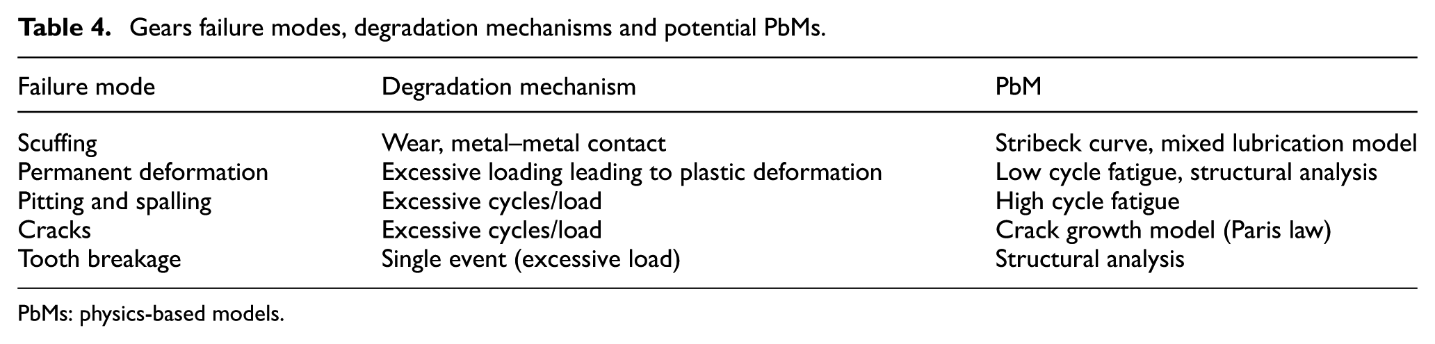
PbMs: physics-based models.

Table 5.

Bearings failure modes, degradation mechanisms and potential PbMs.

Failure mode	Degradation mechanism	PbM
Inner/outer/ball failure (rolling bearing only)	Wear	Fundamental frequencies model to identify faulty sub-component
Spalling/pitting/cracks	Excessive cycles/load	Spalling growth estimation model/stiffness model changes in frequency spectrum
Insufficient lubrication	Wear, metal–metal contact	Stribeck curve, mixed lubrication model

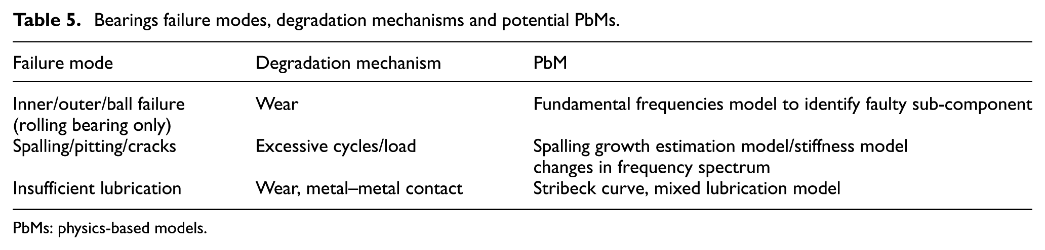
PbMs: physics-based models.

Relevant degradation models

The importance of representing accurately the physics of the system has already been mentioned in previous sections. This section reviews the models of the most relevant degradation mechanisms of rotating machinery. Common failure modes of rotating machinery and their corresponding degradation mechanisms were identified. The aim of this section is to serve as a tool to select the most appropriate models to represent these mechanisms. Additionally, the understanding of the most critical variables and parameters of each degradation mechanism will help to identify what phenomena should be monitored. The following degradation mechanisms are covered:

Creep;

Fatigue;

Fatigue and creep;

Wear.

The amount of health condition monitoring algorithms based on PbMs is limited, as opposed to DDMs. PbMs are not scalable between different systems; additionally, they require a good understanding of the phenomena behind a failure mode. However, health monitoring using PbM is particularly useful in prognostic algorithms due to their potential to estimate the current and future health of the system based on degradation models. The models described in this section are summarized in Table 6.

Table 6.

Health condition algorithms based on PbMs.

Creep	Fatigue	Creep and fatigue	Wear
Baraldi et al.,^19,44 Chin¹⁰⁵ and Yu and Zhou¹⁰⁶	Fatigue^48,77	Vogel et al.,¹⁰⁷ Daroogheh et al.,¹⁰⁸ Bray et al.,¹⁰⁹ Wu et al.¹¹⁰ and Tinga et al.¹¹¹	General wear¹¹²
	Cracks^{14,28–32,113,114}		Fretting^115–118
	Spalling^{35,37,119–123}		Metal–metal contact^46,124,125

PbMs: physics-based models.

Creep

Creep consists of a permanent deformation that can be caused by low loads under high temperature due to the formation of voids in the grain boundaries (GBs) of the material that extends until it becomes inter-granular and fracture occurs. The creep phenomenon is time and temperature dependent. Creep is divided into three stages depending on the creep rate, defined in equation (1), where ε is the deformation and t is the time:¹²⁶

First stage: initially, there is primary creep, with a decelerating creep rate.

Second stage: stable minimum creep rate, called secondary creep, which covers most of the time.

Third stage: creep rate, called tertiary creep, accelerates until fracture occurs.

Creep rate = \frac{Δ ε}{Δ t}

(1)

The Larson Miller parameter (LMP), shown in equation (2), is commonly used to characterize creep behaviour, reducing the problem from two variables, time and temperature, to only one: the LMP. The correlation between maximum stress and LMP depending on the material can be obtained experimentally. However, this equation is purely experimental and does not rely on the physics of the degradation mechanism. It also implies constant temperature along time. Thus, for variable conditions, a cumulative damage rule is required. For instance, a parameter D can be used if stress and temperature levels vary over time to take into account the damage on each instant as shown in equation (3), where $Δ t_{i}$ is the duration of a constant loading period and $Δ t_{r, i}$ is the rupture time for the given loading condition, obtained from equation (2). The failure is estimated when D is above 1⁶⁰

LMP = (T (° F) + 460) \times (20 + \log_{10} (t)) \times 10^{- 3}

(2)

D = \sum_{i = 1}^{n periods} D_{i} = \sum_{i = 1}^{n periods} \frac{Δ t_{i}}{Δ t_{r, i}}

(3)

Instead of using the LMP, a physics-related model that is commonly used to represent creep behaviour is Norton creep law, as shown in equation (4), where σ is the stress level; T is the temperature; and A, n and p are material constants. It should be noted that Norton creep law is only able to represent the second stage of creep behaviour and does not consider material behaviour at a microscopic level.⁴⁵ More complex models that take into account these effects are able to estimate the first and third stages as well^127,128

Creep rate = A T^{n} σ^{m}

(4)

The application of creep models for health condition monitoring has been focused on hot sections of turbine blades. Chin¹⁰⁵ proposed a prognostic approach that estimates the RUL of turbine blades based on a creep model that estimates the stresses based on temperature and time. A similar approach was applied by Baraldi et al.^19,44 to predict creep degradation of turbine blades based on Norton law and Particle Filter (PF) or a Kalman filter for parameter estimation; however, only simulated data were used. Yu and Zhou¹⁰⁶ proposed a creep model based on FEA and the Kachanov–Rabotnov (K-R) model^129,130 to assess damage of high temperature threaded joins by taking into account the damage due to stress relaxation and reduced preload instead of using permanent deformation as the health indicator.

Fatigue

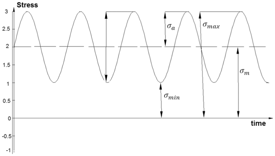
Fatigue occurs in systems subject to cyclic loading, due to thermal and mechanical stresses. The degradation mechanism differs between HCF and LCF. HCF stresses are below the yield stresses and Δσ (stress range) is the factor that controls the degradation mechanism. However, for LCF, the stress level is above the yield stress limit and there is plastic deformation. Thus, Δε (strain range) is the magnitude that controls the degradation.⁴⁵

For HCF, Wöhler¹³¹ demonstrated that the cyclic stress range is the driven factor of fatigue degradation based on experimental fatigue data of railroad axles; thus, it should be represented using S-N curves that correlate the number of cycles and a characteristic stress level. The use of experimental S-N curves can be used for life prediction of metallic structures subject to fatigue. Analytical equations for the appropriate metallic structure can be found in well-accepted standards such as the British Standard 7608:2014,¹³² which also provides the standard deviation as shown in equation (5), where N_f is the number of cycles; $σ_{a}$ is the stress amplitude; SD is the allowed standard deviation; and C_o, d and m are parameters dependent on the geometry.

Apart from the stress range, the mean stress $σ_{m}$ is also an important factor that has to be taken into account, which is normally described as a stress ratio $R = σ_{\max} / σ_{\min}$ . The relation between all these variables is shown in Figure 7.

Figure 7.

Fatigue parameters.

Basquin law¹³³ proposed a stress-based analytical equation based on the experimental work of Wöhler,¹³¹ as shown in equation (6), where N_f also refers to the number of cycles, σ_a is the stress amplitude, $σ'_{f}$ is the fatigue strength coefficient and b is the fatigue strength exponent. It should be noted that any discontinuity in the material, bad surface quality or internal stresses negatively affect the life of the component.⁴⁵ These detrimental factors are particularly critical under high temperatures as shown by Boardman,¹³⁴ who studied the detrimental effect of higher temperature and notches in the fatigue life of a variety of alloys.

\log (N_{f}) = \log (C_{0}) - d \times SD - m \times \log (σ_{a})

(5)

σ_{a} = \frac{Δ σ}{2} = σ'_{f} (2 N_{f})^{b}

(6)

For LCF, plastic deformation is the main factor that controls the failure mechanism; Manson–Coffin law is commonly used to represent this degradation mechanism.^135,136 This method considers that cyclic life depends on the deformation using a power law as shown in equation (7), where $Δ ε_{p}$ is the plastic strain range and c and $ε_{f}$ are experimental constants. A more accurate model, the Manson and Halford model, considers the elastic and plastic component of the strain, thus being able to represent LCF and HCF degradation mechanisms, as shown in equation (8), where D represents the ductility, $σ_{u}$ is the ultimate tensile strength and E is the Young’s modulus.¹²⁶ Kacprzynski et al.⁷⁶ evaluated the plastic strain of a helicopter gear tooth using an FEA model and later applies Manson–Coffin law to evaluate the number of cycles until crack initiation occurs.

Δ ε_{a} = \frac{Δ ε_{p}}{2} = ε_{f} (2 N_{f})^{c}

(7)

Δ ε = D^{0.6} \times N_{f}^{- 0.6} + (\frac{3.5 \times σ_{u}}{E}) \times N_{f}^{- 0.12}

(8)

A cumulative damage rule is required to take into account variable loading conditions. The simplest and a well-accepted approach were proposed by Miner,¹³⁷ as shown in equation (9), where D is the cumulative damage, $n_{i}$ are the current number of cycles under the actual loading condition and $N_{i}$ are the number of cycles until failure, which is estimated if D is above 1. It should be noted that this approach considers the RUL independent of the order of the loads. Similar equations can be used to represent different types of cumulative damage. For instance, Qiu et al.⁴⁸ proposed a similar cumulative rule that is a function of the stiffness of the system instead of the number of cycles

D = \sum_{i = 1}^{load p} \frac{n_{i}}{N_{i}}

(9)

Cracks are a common consequence of fatigue damage, and the degradation mechanism that ultimately leads to failure due to fracture of the component. The previous models do not consider the physics that lead to the fracture and only rely on empirical results. An alternative approach is to predict the failure based on fracture mechanics. Crack growth is divided into three regions:⁴⁵

First region: slow crack growth and the crack length is not considered significant;

Second region: the crack growth rate becomes significant and constant;

Third region: the crack becomes unstable and the propagation rate increases until fracture occurs.

The initial length and the propagation rate of the crack can be estimated and used as an indicator of the RUL of a system subject to fatigue. The most widely accepted model for crack growth, the Paris law, was proposed based on experiments that proved the correlation between crack length and number of cycles by Paris et al.,²⁷ as shown in equation (10), where a is the crack length; N is the number of cycles; m and b are parameters of the material; and K is an intensity coefficient that depends on the geometry and type of crack. A similar equation introduced by Hoeprich¹²¹ can be used to represent spall area growth in bearings, as shown in equation (11), where D is the defect area, C₀ and n material parameters, validated with experimental results by Li et al.¹²² and further improved to consider thermal effects by Kotzalas and Harris.¹²³ It should be noted that specific degradation models can also be used for prognostics. For instance, the rolling contact fatigue model proposed by Sadeghi et al.¹³⁸ based on the crack propagation and crack initiation has the potential to be used for PHM

\frac{da}{dN} = m Δ K^{b}

(10)

\frac{dD}{dN} = C_{0} D^{n}

(11)

Paris law represents the second region of crack growth but does not take into account the initial crack length and the instability of the crack. However, for PHM, being able to represent only the second region of the crack growth using Paris law has proven sufficient to model the degradation of the system. This is shown by Corbetta et al.,²⁸ who estimated the crack growth on structures and the uncertainty of the prediction combining the PbM with PF for parameter estimation. Ray and Tangirala²⁹ also estimated the RUL based on Paris law but using a Kalman filter for parameter estimation. Orchard et al.³⁰ applied both PF and an extended Kalman filter (EKF) on a crack growth model based on Paris law to estimate crack length in the plate of the gearbox of a helicopter. Pais and Kim¹¹⁴ developed a fatigue crack growth PbM for prognostics of aerospace panels by computing a FEA model and a fatigue crack growth model as a function of the usage history, a modified Paris law to consider variable amplitude loads was used.

Zio and Di Maio¹⁴ combined Paris law with a SVM algorithm to select the appropriate degradation model to estimate crack length. Oppenheimer and Loparo³¹ also calculated the RUL of rotor shafts due to cracks using Paris law, while Li and Lee³² combined a dynamic model that estimates the stresses on a gear with Paris law to represent the degradation to estimate the RUL of the gear. A more sophisticated algorithm is proposed by Kacprzynski et al.,⁷⁶ who estimated the RUL of helicopter gears by modelling the first region (crack initiation) using Manson–Coffin law presented above to estimate the number of cycles until a crack initiates and using Paris law to estimate the crack growth afterwards. The spall degradation formula presented in equation (11) has been applied for RUL estimation of rolling bearings by Orsagh et al.³⁴ and Li et al.,^36,37 while Slack and Sadeghi¹²⁰ developed a more sophisticated explicit finite element (FE) spalling model that predicts the number of cycles until failure by modelling the crack initiation in the sub-surface and its propagation. For diagnostics, Fu and Gao¹¹³ developed a PbM capable of estimating the natural frequency response of a crack in a fan blade assessing its size and location.

Creep and fatigue

When alternative loads are coupled with creep deformation, both degradation mechanisms, creep and fatigue, interact with each other and cannot be treated independently.⁴⁵ The most relevant method to represent this behaviour is strain range partitioning (SRP).¹³⁹ The SRP method assumes that different strain ranges produce different hysteresis loops and differentiates between two types of deformation: GB sliding and attendant slip plane (SP) sliding; the former is considered when creep is the main failure mechanism and applies to slow cycles, and the latter applies to degradation caused mainly by fatigue, consisting of deformation due to cyclic loading.¹²⁶ Depending on the type of the strain during the tension and compression phase of the hysteresis loop, four possible scenarios can occur as shown in Figure 8. Once the scenario is identified, the number of cycles to failure can be obtained as a function of the strain range. Vogel et al.¹⁰⁷ used the SRP method to predict crack initiation in a jet engine’s combustor liner and correlate them with experimental results.

Figure 8.

Four SRP hysteresis scenarios: (a) PP, (b) PC, (c) CP, (d) CC, where P refers to plastic strain and C refers to creep strain during tension and compression phases.

However, the SRP method is not the only valid approach. Daroogheh et al.¹⁰⁸ modelled the creep–fatigue behaviour of turbine blades considering both mechanisms independent of each other and calculated the cumulative damage using the rain flow method. Bray et al.¹⁰⁹ used a FEA approach that incorporates creep and fatigue routines to calculate damage in pipe joints. Complex models that take into account the microstructure of the material can also be used to obtain more accurate results as the framework proposed by Wu et al.¹¹⁰ Tinga et al.¹¹¹ developed a degradation model of creep–fatigue that estimated the number of cycles until failure for single crystal Ni-based alloys, obtaining adequate agreement with experimental results.

Wear

Wear, also referred to as abrasion and scuffing, is a degradation mechanism caused by friction between two sliding surfaces associated with loss of material, including damage due to direct contact between the surfaces and damage caused by the fluid between the surfaces.⁴⁵ However, the modelling of wear is particularly challenging due to the high influence of external factors that affect the contact such as the environment.¹¹⁸ Wear can also be considered as a dissipation of energy mainly controlled by friction,¹⁴⁰ and it is classified as follows: adhesive and abrasive (depending on the hardness of the materials in contact¹⁴¹), corrosive, thermal and fatigue wear.¹¹²

Adhesive wear can be modelled using Archard’s law, as shown in equation (12), where $V_{wear}$ is the wear volume, H is the material hardness, W is the load, L is the sliding distance and K is the wear coefficient. Using this law, more complex wear models can be obtained by modifying the value of the constant K, as shown by Watson et al.,¹¹² who applied variants of Archard’s law to represent adhesive, abrasive and corrosive wear

V_{wear} = K (\frac{WL}{3 H})

(12)

Fatigue wear leads to cracks initiated below the surface. After a number of cycles these cracks develop into pitting or spalling with the subsequent removal of material. A degradation model for wear caused by sub-surface fatigue has been proposed by Ghosh et al.,¹⁴² who provided an experimental correlation between wear and crack propagation, which is a function of the shear stress on the surface as shown in equation (13), where N is the number of cycles to failure; a and b are empirical constants; and Q is the contact shear stress that depends on the friction coefficient and load applied

\log (N) = a \cdot \log (Q) + b

(13)

However, wear is controlled by Friction. Therefore, more accurate models should predict the friction between the sliding surfaces as well. The friction force is defined as the opposing force to the motion of a body to another and depends on the normal force and the friction coefficient. For non-lubricated contacts, Coulomb law¹⁴³ can be applied, considering the friction coefficient constant and independent of the speed and load, as shown in equation (14). Where F_T is the friction force, µ is the friction coefficient and F_N is the normal force, but for lubricated contact in motion hydrodynamic theory must be applied

F_{T} = μ F_{N}

(14)

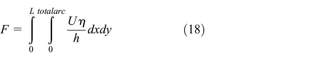
For lubricated sliding contacts, the friction is divided into four regions depending on the type of contact as shown in Figure 9: hydrodynamic lubrication, elasto-hydrodynamic lubrication (EHL), mixed lubrication and boundary lubrication, where the friction coefficient is represented as a function of a lubrication parameter, the Sommerfeld number S, which includes the effect of speed, load and viscosity.

Figure 9.

Qualitative Stribeck curve: friction (µ), Sommerfeld number (N: speed, p: load, η: dynamic viscosity of the lubricant, R: radius of the bearing, c: clearance of the bearing).

Hydrodynamic contacts in rotating machinery, typically rolling and hydrodynamic bearings, are designed to operate on the hydrodynamic region, where the contact is fully lubricated and the friction forces are exclusively caused by the shear stresses of the lubricant. The fluid can be considered laminar and a simplified version of the Reynolds equation¹⁴⁴ using dimensionless parameters can be integrated along the bearing to calculate the film thickness and pressure distribution as shown in equation (15), where $h^{*}$ is the dimensionless film thickness, $p^{*}$ is the dimensionless pressure, $x^{*}$ is the radial coordinate, $y^{*}$ is the axial coordinate; and R and L are the dimensionless radius and length, respectively.¹⁴⁵ The friction force is calculated by integrating the shear stress $τ$ along the bearing area as shown in equation (16), which requires the lubricant speed gradient on the surface, as shown in equation (17), thus obtaining the friction force as a function of the film thickness (18), where U is the relative speed and $η$ is the dynamic viscosity

\frac{\partial}{\partial x^{*}} (h^{* 3} \frac{\partial p^{*}}{\partial x^{*}}) + {(\frac{R}{L})}^{2} \frac{\partial}{\partial y^{*}} (h^{*} \frac{\partial p^{*}}{\partial y^{*}}) = \frac{\partial h^{*}}{\partial x^{*}}

(15)

F = \int_{0}^{L} \int_{0}^{total arc} τ dxdy = \int_{0}^{L} \int_{0}^{total arc} η \frac{\partial u}{\partial z} dxdy

(16)

\frac{\partial u}{\partial z} = \frac{U}{h}

(17)

F = \int_{0}^{L} \int_{0}^{total arc} \frac{U η}{h} dxdy

(18)

For plain journal bearings, the film thickness h can be obtained as a function of the geometry and the eccentricity ratio ε, as shown in equation (19), where c is the clearance and θ is the radial angle. Thus, an analytical solution of the Reynolds equation (15) is obtained (equation (20)), where p is the pressure distribution as a function of the radial angle θ, the relative speed between the sliding surfaces U, the eccentricity ratio ε, the axial position y, the dynamic viscosity η and geometrical parameters: radius R, clearance c and bearing length L. The friction force can be obtained analytically as shown in equation (21).¹⁴⁵ Alternatively, Sinanoglu et al.¹⁴⁶ successfully estimated the pressure variations of a journal bearing using an ANN, but several pressure sensors along the bearing were required to train the network

h (θ) = c (1 + ε \cdot \cos (θ))

(19)

p = \frac{3 \cdot U \cdot η \cdot \sin (θ)}{R \cdot c^{2} {(1 + ε \cdot \cos (θ))}^{3}} (\frac{L^{2}}{4} + y^{2})

(20)

F = \frac{2 π η U L R}{c \sqrt{(1 - ε^{2})}}

(21)

The EHL regime applies under heavily loaded conditions. The deformation of the bearings caused by the load significantly affects the film thickness and should be considered by the model. Thus, a structural analysis is required to calculate the radial deformation along the bearing $d (θ, y)$ caused by the pressure filed and should be included in the calculation of the film thickness as shown in equation (22). EHL models have been used for estimating the minimum film thickness based on operational conditions, as shown by Choi et al.,¹⁴⁷ who combined a multi-flexible dynamic model of the bearing with an EHL model that calculates the pressure distribution and film thickness

h (θ, y) = c (1 + ε \cdot \cos (θ)) + d (θ, y)

(22)

An alternative approach is to use computational fluid dynamics (CFD) for hydrodynamic lubrication and to combine it with computational structural analysis for EHL. Stefani and Rebora¹⁴⁸ developed a CFD model that takes into account the wall convection, the thermo-mechanical deformations and the mixing phenomena in the groove, while Jin and Zuo¹⁴⁹ also used a CFD model to study the effect of different groove depths in journal bearings.

Mixed lubrication refers to the region in which partial metal–metal contact occurs and part of the load is transmitted by asperities. In this situation, surface parameters must be taken into account and the complexity and quantity of unknown parameters increase. Gelinck and Schipper¹⁵⁰ have developed a mixed lubrication model for line contacts which was later improved and validated for point contacts by Liu,¹⁵¹ and which agreed with experimental results as shown by Lu et al.¹⁵² The mixed lubrication model first calculates the film thickness and applies the mixed lubrication model if h < h_lim is true; otherwise, the contact is considered hydrodynamic, h being the minimum film thickness and h_lim the limit at which mixed lubrication occurs. The mixed lubrication model assumes a percentage of the load transmitted through asperities, $δ_{2}$ , and compares the pressure distribution transmitted through the asperities with the pressure distribution considering a Hertzian contact; $δ_{2}$ is updated until equation (23) converges, where F_3/2 is illustrated in equation (24), $\bar{n}$ is the dimensionless density of asperity summits, ${\bar{σ}}_{s}$ is the dimensionless standard deviation of the asperity height distribution, W is the load, A is the apparent contact area, p_max is the maximum Hertzian pressure and $Φ_{s}^{*}$ is the standardized Gaussian distribution

\frac{2}{3} \bar{n} {\bar{σ}}_{s}^{3 / 2} F_{3 / 2} (\frac{h}{{\bar{σ}}_{s}}) = \frac{W}{A δ_{2} p_{\max}}

(23)

F_{\frac{3}{2}} (φ) = \int_{φ}^{\infty} (s - φ)^{\frac{3}{2}} Φ_{s}^{*} (s) ds

(24)

The Greenwood and Williamson¹⁵³ asperity contact model was used to calculate the load transmitted through the asperities, by considering spherical summits with a height that follows a Gaussian distribution subject to elastic deformation.

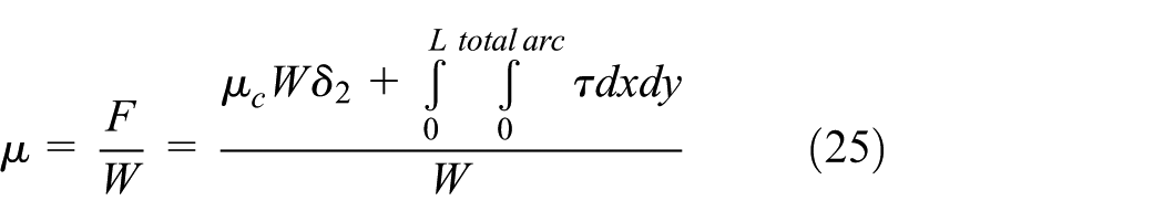
Under mixed lubrication, the friction coefficient is calculated as a function of the shear stress of the lubricant for the load transmitted through the lubricant (equation (16)) and using Coulomb law (equation (14)) for the load transmitted through the asperities as shown in equation (25), where $μ$ is the friction coefficient, $μ_{c}$ is the friction coefficient for a dry contact, F is the friction force, W is the load and $τ$ is the shear stress of the lubricant

μ = \frac{F}{W} = \frac{μ_{c} W δ_{2} + \int_{0}^{L} \int_{0}^{total arc} τ dxdy}{W}

(25)

Faraon¹⁵⁴ presented a similar approach for line contacts further improved for starved contacts by Faraon and Schipper.¹⁵⁵ For point contact, Hua et al.¹⁵⁶ developed a mixed lubrication model that calculates the film thickness, pressure and temperature along the contact considering conductive thermal effects and stated the potential of the mixed lubrication model for scuffing prediction. Hu and Zhu¹⁵⁷ did not take into account the thermal effects but included the surface deformation in the calculation of the film thickness for EHL and mixed lubrication. A similar approach was used to detect scuffing in gears using a mixed lubrication model by Castro and Seabra.⁴⁶ Wang et al.¹⁵⁸ developed a mixed lubrication model that evaluates the influence of misalignment in hydrodynamic bearings under severe conditions that was validated using temperature data and stresses the influence of surface parameters when the film thickness is of the same order of magnitude as the roughness of the surface. Under boundary conditions, the lubricant does not transmit any of the load, and Coulomb and dry contact models are more suitable.

Stribeck curve modes can be applied to any lubricated contact, point contact models are normally used for ball rolling bearings, whereas line contact models are used for hydrodynamic and roller bearings. However, Wang et al.¹⁵⁹ developed a Stribeck curve model validated with experimental results for deep-groove ball bearings by calculating the torque produced by elastic hysteresis, hydrodynamic lubrication, slip, and friction between balls, cage and guiding lands using a complete different approach based on the energy lost.

PbMs for PHM based on degradation caused by wear are limited. However, the techniques to model wear presented above have the potential to be applied to PHM. Wear models have been used by Zhang et al.¹⁶⁰ to detect failures in piston bearings as a function of temperature, friction and roughness.

A variant of wear fatigue, called fretting, is associated with the small amplitude oscillatory motion between two solid surfaces in contact.¹¹⁵ Leonard et al.¹¹⁶ modelled a fretting in a line contact and calculate the severity of wear as a function of the number of cycles using Coulomb law (equation (14)) to represent the friction, a FE to represent the stresses and Archard’s law to take into account the cumulative damage. Kasarekar et al.¹¹⁷ evaluated the fretting fatigue life depending on the roughness of the surfaces in contact estimating the crack initiation using the Smith Watson Topper fatigue theory and Archard’s law to model the wear. Quraishi et al.¹¹⁸ also calculated the fretting fatigue life as a function of friction and loading using the Ramberg–Osgood equation and validated it with experimental results, while Walvekar et al.¹¹⁵ also validated a fretting model that consists of a FEA model that computes the stresses and strains during each cycle and uses an exponential law to model the cumulative fatigue damage.

Li and Kahraman^125,161 proposed a PbM to calculate the fatigue life of point contacts due to micro-pitting caused by metal–metal contact that was validated with experimental results by assuming crack propagation negligent compared to clack initiation. However, thermal effects were not considered. Li et al.¹²⁴ experimentally validated a similar model that predicted wear of point contacts, by integrating the calculation of the friction coefficient and a heat transfer model that estimated the friction coefficient and the temperature. Marble and Morton¹¹⁹ validated a degradation model for wear caused by spalling in rolling bearings as a function of the area of the defect, the load and material constants. Watson et al.¹¹² developed an algorithm capable of predicting the RUL of clutches by combining a dynamic model of the system and wear degradation models based on Archard’s law presented above taking into account corrosive, adhesive and abrasive wear.

Discussion

In the previous sections, the most common failure modes of gears and bearings of rotating machinery were reviewed with focus on the PHM methods for each failure mode. Special attention was given to the PbM approaches available in the literature. The corresponding degradation mechanisms and PbMs were identified and the potential degradation models presented.

The use of PbMs, particularly for prognostics, has some advantages when compared to DDMs. However, to choose between one or the other, each failure mode has to be analysed independently. As shown in previous sections, many relevant failure modes are not suitable for a PbM approach, because the physics of failure cannot be modelled or because even if the degradation was modelled successfully, the inputs of those models would be unknown. Misalignment, geometrical errors or dirt are common failure modes for which PbMs are particularly challenging.

Another additional difficulty of using PbMs for PHM is the necessary understanding of the physics of failure. If enough data are available, DDM can provide a correlation between the measured variables of a system and its health without further analysis of the physics of failure; moreover, if PHM is developed in a variety of systems and failure modes, DDM approaches are scalable, because each system and failure mode does not require a deep analysis of the phenomena as opposed to PbM approaches.

However, large data sets of healthy and faulty conditions are not always available; besides, if new sensors are incorporated, information about their readings would not be available, which means that in many cases additional testing would be needed. An additional aspect, particularly for prognostics, is that DDMs require a significant amount of faulty data sets, but for high valuable assets, for example, aerospace, the failure rate is normally low and faulty data sets are rare.

The necessary understanding of the physics of failure of PbM approaches can be considered as a drawback due to the additional effort and expertise required, but also as an opportunity, because it provides an algorithm based on physical principles in which the relation between the PbM inputs and the health of the system is well understood; thus, the reasoning and health indicators have a physical meaning. A PbM can be modelled with shorter data sets than DDMs, because data are needed for adjusting the parameters and validating the model, whereas DDMs, particularly those based on artificial intelligence, require training data, validation data and are subject to overfitting. In addition, the knowledge about the physics of failure has synergies with the design process and can facilitate the certification, because the principles behind the algorithm are be justified by proven physical principles.

On one hand, DDMs can be used for diagnostics and prognostics, but their architecture is different. For diagnostics, the algorithm should distinguish between two states (healthy and unhealthy), whereas for prognostics the algorithm should identify the degree of degradation and its future heath values, making prognostics particularly challenge for DDMs. On the other hand, PbMs can also be used for diagnostics and prognostics, but for prognostics the assessment of the degree of degradation in the present and future is defined by the degradation model, which is the reason why PbMs are particularly suitable for prognostics. However, the degradation estimated by a PbM differs from the real degradation of the system. If there is an additional way of assessing the degree of degradation, for example, a sensor measuring the temperature of a bearing, directly related to the friction due to metal–metal contact, then a parameter estimator can be used to correct the model parameters and adjust the estimated RUL.

Different degradation models commonly used in rotating machinery have been presented, from simple analytical equations to complex models based on CFD and FEA. All the inputs of a degradation model should be monitored or estimated, which means that when deciding which model should be used, even if a more complex model apparently is more accurate, a simpler model with less inputs and parameters may provide similar results if most of its inputs and parameters must be estimated. The computational time and memory are limited, which can be an additional drawback of using more complex models.

Creep models have been proposed for PHM using the Norton law that relates the deformation as a function of time and temperature. The proposed PbMs have the potential to be used in the future for prognostics of components subject to high temperatures. Fatigue is one of the best known degradation mechanisms. The majority of PbMs for prognostics are based on fatigue principles, either using HCF and LCF models or modelling the crack growth. Therefore, failure modes mainly caused by fatigue are ideal candidates for PbM approaches due to the extensive literature and options available.

In systems subject to mechanical stresses and high temperature, the degradation is caused by fatigue and creep. However, both degradation mechanisms are coupled and cannot be considered independent of each other. The correlation between fatigue and creep is understood and there are PbMs for prognostics in combustor liners and turbine blades, but they are more complex than fatigue or creep models.

Wear is a broad degradation mechanism and the physics behind it differ between dry and lubricated contacts. Dry contacts and fretting are normally modelled using analytical equations but depend on empirical parameters. Prognostics PbMs have been proposed based on wear in dry contacts; however, lubricated contacts are more relevant in rotating machinery.

Wear in lubricated contacts is minimized due to the lubricant film; this film is produced by the relative motion between the surfaces. Under normal condition, wear is negligible, but if the film cannot transmit the load partial metal–metal occurs with the subsequent degradation. The physics of failure are complex because hydrodynamic, mechanical and thermal phenomena are coupled; however, there are several PbMs capable of modelling this degradation mechanism. However, few health condition monitoring algorithms have been proposed.

Conclusion

The area of PbM for health condition monitoring of rotating machinery has been reviewed in this article including the most common parameter estimator techniques and failures modes of rotating machinery along with the models available to represent their degradation mechanisms.

Although comprehensive review papers on PHM for rotating machinery are available, approaches based on PbM have not been extensively reviewed in comparison with DDM approaches. The development of a PHM system based on the physics of the system requires a good understanding of the failure modes and their degradation mechanisms. This article aims to serve as a tool to identify common failure modes and their corresponding degradation mechanisms, and to provide a review of the models available to represent the degradation for prognostics based on PbMs.

Rotating machinery components are subject to a variety of failure modes. Although diagnostics for rotating machinery has been extensively studied, research in prognostics is more limited. Vibration analysis and AEs are the main diagnostics and prognostics techniques for gears. PbM approaches commonly consist of a dynamics model of the system that correlates the vibration signal with the stresses plus a crack growth model that estimates the RUL.

In rolling bearings, vibration and AE along with temperature analysis are the most common techniques. PbMs have been applied using a degradation formula similar to Paris law to represent spalling or the identification of the natural frequencies of each rotating component and the amplitude of their response for fault identification and fault isolation. It should also be noted that promising results using AE compared to vibration analysis rely on a high S-N ratio.

Research in PHM for hydrodynamic bearings is more limited. Most of the research focuses on detecting metal–metal contact using temperature, vibration analysis, AEs or metallic particle measurement using DDM approaches. However, the hydrodynamic phenomena are well understood and there are models available, but the potential of these models has not been used for health condition monitoring.

Even if PbMs for PHM have the potential to obtain more accurate predictions, they are not suitable for every system and failure mode. The following limitations of applying PbMs for diagnostics and prognostics should be taken into account:

Some degradation mechanisms cannot be modelled; thus, PbMs cannot be developed.

PbM algorithms are not scalable between different systems as opposed to DDM algorithms.

Expert knowledge is required.

Additional measurement of the health is preferable to minimize prognosis errors.

However, prognostics PbM approaches have several advantages that can make them ideal for certain systems and failure modes:

Large data sets are not required as opposed to DDMs.

Understanding of the system and the physics of failure may be used in other areas (design) and is easily justified for certification purposes.

Health indicators based on degradation models have a physical meaning.

The prognostics architecture based on PbMs is defined by the degradation model, whereas prognostics DDMs have complex architectures to identify the current and future degree of degradation.

After this review, it has been shown that relatively simple formulas, for example, creep and fatigue models, can be easily implemented for prognostics based on PbM, while more complex formulas may also be used for more accurate predictions or for complex phenomena where different physics are involved, for example, creep in combination with fatigue or hydrodynamic lubrication combined with metal–metal contact. For more precise results sophisticated models can be used, for example, numerical methods such as FEA or CFD analysis, or models that take into account the micro-structure of the material for creep.

It should be noted that a more complex model would led to more accurate predictions assuming that all the parameters required by the model are known. However, the number of sensors is limited and certain parameters can only be estimated; thus, less accurate than if all the parameters are well known. For the design of prognostics capabilities, it may be preferable to develop simple models with measurable parameters instead of complex models that require several assumptions and estimated values. This is due to the following reasons: the accuracy may not be significantly increased if many parameters are estimated, and more complex models require more computational power, which could be a limiting factor in the design of PHM solutions.

Footnotes

Academic Editor: Michal Kuciej

Declaration of conflicting interests

The author(s) declared no potential conflicts of interest with respect to the research, authorship and/or publication of this article.

Funding

The author(s) disclosed receipt of the following financial support for the research, authorship and/or publication of this article: The research leading to these results has received funding from the European Union Seventh Framework Programme (FP7/2007-2013) under Grant Agreement No. 605779 (project RepAIR). The text reflects the authors’ views. The European Commission is not liable for any use that may be made of the information contained therein. For further information, see . Adrian Uriondo – Proof reading and advice.

References

Kothamasu

Huang

Verduin

WH.

System health monitoring and prognostics – a review of current paradigms and practices. Int J Adv Manuf Tech 2006; 28: 1012–1024.

Jennions

IK.

Integrated vehicle health management: perspectives on an emerging field. Warrendale, PA: SAE International, 2011.

MacConnell

. ISHM & design: a review of the benefits of the ideal ISHM system. In: Proceedings of the 2007 IEEE aerospace conference, Seattle, WA, 3–10 March 2007, pp.1–18. New York: IEEE.

Baroth

Powers

Fox

. IVHM (Integrated Vehicle Health Management) techniques for future space vehicles. In: Proceedings of the 37th joint propulsion conference and exhibit 2001, Salt Lake City, UT, 8–11 July 2011, pp.1–10. AIAA.

Sikorska

Hodkiewicz

Prognostic modelling options for remaining useful life estimation by industry. Mech Syst Signal Pr 2011; 25: 1803–1836.

Lee

Zhao

. Prognostics and health management design for rotary machinery systems – reviews, methodology and applications. Mech Syst Signal Pr 2014; 42: 314–334.

Engel

Gilmartin

Bongort

. Prognostics, the real issues involved with predicting life remaining. In: Proceedings of the IEEE aerospace conference proceedings, Big Sky, MT, 18–25 March 2000, vol. 6, pp.457–470. New York: IEEE.

Eker

Camci

Jennions

. Major challenges in prognostics: study on benchmarking prognostics datasets. In: Proceedings of the PHM, Dresden, 3–5 July 2012, vol. 3, pp.1–8. PHM Society.

Heng

Zhang

Tan

ACC

. Rotating machinery prognostics: state of the art, challenges and opportunities. Mech Syst Signal Pr 2009; 23: 724–739.

10.

Luo

Namburu

Pattipati

. Model-based prognostic techniques [maintenance applications]. In: Proceedings of the IEEE systems readiness technology conference (AUTOTESTCON 2003), Anaheim, CA, 22–25 September 2003, pp.330–340. New York: IEEE.

11.

Liang

Time–frequency signal analysis for gearbox fault diagnosis using a generalized synchrosqueezing transform. Mech Syst Signal Pr 2012; 26: 205–217.

12.

Mu-jun

Shi-Yong

. Fault diagnosis of air compressor based on RBF neural network. In: Proceedings of the 2011 international conference on mechatronic science, electric engineering and computer (MEC), Jilin, China, 19–22 August 2011, pp.887–890. New York: IEEE.

13.

Ferreiro

Arnaiz

Sierra

. Application of Bayesian networks in prognostics for a new Integrated Vehicle Health Management concept. Expert Syst Appl 2012; 39: 6402–6418.

14.

Zio

Di Maio

Fatigue crack growth estimation by relevance vector machine. Expert Syst Appl 2012; 39: 10681–10692.

15.

Pantelelis

Kanarachos

Gotzias

Neural networks and simple models for the fault diagnosis of naval turbochargers. Math Comput Simulat 2000; 51: 387–397.

16.

Saxena

Saad

Evolving an artificial neural network classifier for condition monitoring of rotating mechanical systems. Appl Soft Comput 2007; 7: 441–454.

17.

Chong

K-T.

Induction machine condition monitoring using neural network modeling. IEEE T Ind Electron 2007; 54: 241–249.

18.

Reda Taha

Lucero

. Damage identification for structural health monitoring using fuzzy pattern recognition (SEMC 2004 structural health monitoring, damage detection and long-term performance; Second international conference on structural engineering, mechanics and computation). Eng Struct 2005; 27: 1774–1783.

19.

Baraldi

Mangili

Zio

A Kalman filter-based ensemble approach with application to turbine creep prognostics. IEEE T Reliab 2012; 61: 966–977.

20.

Polikar

Ensemble based systems in decision making. IEEE Circ Syst Mag 2006; 6: 21–45.

21.

Jardine

AKS

Lin

Banjevic

A review on machinery diagnostics and prognostics implementing condition-based maintenance. Mech Syst Signal Pr 2006; 20: 1483–1510.

22.

Lei

Lin

. A review on empirical mode decomposition in fault diagnosis of rotating machinery. Mech Syst Signal Pr 2013; 35: 108–126.

23.

Sait

Sharaf-Eldeen

YI.

A review of gearbox condition monitoring based on vibration analysis techniques diagnostics and prognostics, vol. 5 (Proceedings of the society for experimental mechanics series). New York: Springer, 2011, pp.307–324.

24.

Kim

Choi

. Options for prognostics methods: a review of data-driven and physics-based prognostics. In: Proceedings of the 54th AIAA/ASME/ASCE/AHS/ASC structures, structural dynamics, and materials conference, Boston, MA, 8–11 April 2013, pp.1–14. Reston, VA: AIAA.

25.

Luo

Bixby

Pattipati

. An interacting multiple model approach to model-based prognostics. In: Proceedings of the 2003 IEEE international conference on systems, man and cybernetics, Washington, DC, 5–8 October 2003, vol. 1, pp.189–194. New York: IEEE.

26.

Chow

M-Y

Tipsuwan

. Neural-network-based motor rolling bearing fault diagnosis. IEEE T Ind Electron 2000; 47: 1060–1069.

27.

Paris

Gomez

Anderson

WE.

A rational analytic theory of fatigue. Trend Eng 1961; 13: 9–14.

28.

Corbetta

Sbarufatti

Manes

. Sequential Monte Carlo sampling for crack growth prediction providing for several uncertainties. In: Proceedings of the 2nd European conference of the prognostics and health management society 2014, Nantes, 8–10 July 2014, vol. 5, pp.1–13. PHM Society.

29.

Ray

Tangirala

Stochastic modeling of fatigue crack dynamics for on-line failure prognostics. IEEE T Contr Syst T 1996; 4: 443–451.

30.

Orchard

Kacprzynski

Goebel

. Advances in uncertainty representation and management for particle filtering applied to prognostics. In: Proceedings of the prognostics and health management international conference, Denver, CO, 6–9 October 2008, pp.1–6. New York: IEEE.

31.

Oppenheimer

Loparo

. Physically based diagnosis and prognosis of cracked rotor shafts. In: Proceedings of the components and systems diagnostics, prognostics, and health management II, Orlando, FL, 1 April 2002, pp.122–132. Bellingham, WA: SPIE.

32.

Lee

Gear fatigue crack prognosis using embedded model, gear dynamic model and fracture mechanics. Mech Syst Signal Pr 2005; 19: 836–846.

33.

Coppe

Pais

Kim

N-H

. Identification of equivalent damage growth parameters for general crack geometry. In: Proceedings of the annual conference of the prognostics and health management society, Portland, OR, 10–16 October 2010, pp.1–10. PHM Society.

34.

Orsagh

Sheldon

Klenke

. Prognostics/diagnostics for gas turbine engine bearings. In: Proceedings of the 2003 IEEE aerospace conference, Big Sky, MT, 8–15 March 2003, pp.3095–3103. New York: IEEE.

35.

Jaw

Wang

. Mathematical formulation of model-based methods for diagnostics and prognostics. In: Proceedings of the 2006 ASME 51st turbo expo: power for land, sea, and air, Barcelona, 8–11 May 2006, pp.691–697. New York: ASME.

36.

Kurfess

Liang

SY.

Stochastic prognostics for rolling element bearings. Mech Syst Signal Pr 2000; 14: 747–762.

37.

Billington

Zhang

. Adaptive prognostics for rolling element bearing condition. Mech Syst Signal Pr 1999; 13: 103–113.

38.

Simon

A comparison of filtering approaches for aircraft engine health estimation. Aerosp Sci Technol 2008; 12: 276–284.

39.

Wagner

Shoureshi

. A robust failure diagnostics scheme for nonlinear thermofluid processes. In: Proceedings of the 1987 American control conference, Minneapolis, MN, 10–12 June 1987, pp.1877–1882. New York: IEEE.

40.

Laroche

Sedda

Durieu

Methodological insights for online estimation of induction motor parameters. IEEE T Contr Syst T 2008; 16: 1021–1028.

41.

Simani

Identification and fault diagnosis of a simulated model of an industrial gas turbine. IEEE T Ind Inform 2005; 1: 202–216.

42.

Peel

. Data driven prognostics using a Kalman filter ensemble of neural network models. In: Proceedings of the 2008 international conference on prognostics and health management (PHM 2008), Denver, CO, 6–9 October 2008, pp.1–6. New York: IEEE.

43.

Saha

Goebel

Christophersen

Comparison of prognostic algorithms for estimating remaining useful life of batteries. T I Meas Control 2009; 31: 293–308.

44.

Baraldi

Cadinia

Mangilia

. Prognostics under different available information. Chem Eng 2013; 33: 163–168.

45.

Tinga

Principles of loads and failure mechanisms: applications in maintenance, reliability and design. London: Springer Science & Business Media, 2013.

46.

Castro

Seabra

Global and local analysis of gear scuffing tests using a mixed film lubrication model. Tribol Int 2008; 41: 244–255.

47.

McFadden

Toozhy

MM.

Application of synchronous averaging to vibration monitoring of rolling element bearings. Mech Syst Signal Pr 2000; 14: 891–906.

48.

Qiu

Seth

Liang

. Damage mechanics approach for bearing lifetime prognostics. Mech Syst Signal Pr 2002; 16: 817–829.

49.

Warren

Guo

YB.

Acoustic emission monitoring for rolling contact fatigue of superfinished ground surfaces. Int J Fatigue 2007; 29: 603–614.

50.

Rahman

Ohba

Yoshioka

. Incipient damage detection and its propagation monitoring of rolling contact fatigue by acoustic emission. Tribol Int 2009; 42: 807–815.

51.

Hort

Mazal

Vlasic

Monitoring of acoustic emission signal of loaded axial bearings. J Mater Sci Eng A: Struct Mater Prop Microstruct Process 2010; 1: 717–724.

52.

Hort

Mazal

Application of acoustic emission for measuring of contact fatigue of axial bearing. Eng Mech 2011; 18: 117–125.

53.

Elforjani

Mba

Observations and location of acoustic emissions for a naturally degrading rolling element thrust bearing. J Fail Anal Prev 2008; 8: 370–385.

54.

Guo-Lu

Zhi-Qiang

Hai-Dou

. Acoustic emission monitoring and failure mechanism analysis of rolling contact fatigue for Fe-based alloy coating. Tribol Int 2013; 61: 129–137.

55.

Sunnersjö

CS.

Rolling bearing vibrations – the effects of geometrical imperfections and wear. J Sound Vib 1985; 98: 455–474.

56.

Sawalhi

Randall

RB.

Vibration response of spalled rolling element bearings: observations, simulations and signal processing techniques to track the spall size. Mech Syst Signal Pr 2011; 25: 846–870.

57.

Zhang

Z-Q

G-L

Wang

H-D

. Investigation of rolling contact fatigue damage process of the coating by acoustics emission and vibration signals. Tribol Int 2012; 47: 25–31.

58.

Price

Lees

Friswell

MI.

Detection of severe sliding and pitting fatigue wear regimes through the use of broadband acoustic emission. Proc IMechE, Part J: J Engineering Tribology 2005; 219: 85–98.

59.

Guo

Schwach

DW.

An experimental investigation of white layer on rolling contact fatigue using acoustic emission technique. Int J Fatigue 2005; 27: 1051–1061.

60.

Tan

Irving

Mba

A comparative experimental study on the diagnostic and prognostic capabilities of acoustics emission, vibration and spectrometric oil analysis for spur gears. Mech Syst Signal Pr 2007; 21: 208–233.

61.

Elasha

Ruiz-Cárcel

Mba

. Pitting detection in worm gearboxes with vibration analysis. Eng Fail Anal 2014; 42: 366–376.

62.

Feng

Liang

Fault diagnosis of wind turbine planetary gearbox under nonstationary conditions via adaptive optimal kernel time–frequency analysis. Renew Energ 2014; 66: 468–477.

63.

Tan

Mba

Identification of the acoustic emission source during a comparative study on diagnosis of a spur gearbox. Tribol Int 2005; 38: 469–480.

64.

Peng

Kessissoglou

An integrated approach to fault diagnosis of machinery using wear debris and vibration analysis. Wear 2003; 255: 1221–1232.

65.

Kim

Y-H

Tan

ACC

Mathew

. Condition monitoring of low speed bearings: a comparative study of the ultrasound technique versus vibration measurements. In: Proceedings of the 1st world congress on engineering asset management (WCEAM), Gold Coast, QLD, Australia, 11–14 July 2006, pp.182–191. London: Springer.

66.

Choudhury

Tandon

Application of acoustic emission technique for the detection of defects in rolling element bearings. Tribol Int 2000; 33: 39–45.

67.

Zhang

Friswell

MI.

Observation of time-frequency characteristics of the acoustic emission from defects in rolling element bearings. Insight 2010; 52: 412–418.

68.

Jamaludin

Mba

Monitoring extremely slow rolling element bearings: part I. NDT&E Int 2002; 35: 349–358.

69.

Jamaludin

Mba

Monitoring extremely slow rolling element bearings: part II. NDT&E Int 2002; 35: 359–366.

70.

Zakrajsek

Lewicki

DG.

Detecting gear tooth fatigue cracks in advance of complete fracture. Tribotest 1998; 4: 407–422.

71.

Park

Youn

. Fault diagnostics of planet gears in wind turbine using autocorrelation-based time synchronous averaging (ATSA). In: Proceedings of the second European conference of the prognostics and health management society 2014, Nantes, 8–10 July 2014, pp.1–8. PHM Society.

72.

Sun

Wood

RJK

Wang

. Wear monitoring of bearing steel using electrostatic and acoustic emission techniques. Wear 2005; 259: 1482–1489.

73.

Harvey

Wood

RJK

Powrie

HEG

. Electrostatic wear monitoring of rolling element bearings. Wear 2007; 263: 1492–1501.

74.

Boness

McBride

SL.

Adhesive and abrasive wear studies using acoustic emission techniques. Wear 1991; 149: 41–53.

75.

Feng

Zuo

Hao

. Gear crack assessment based on cyclic correlation analysis. In: Proceedings of the 8th international conference on reliability, maintainability and safety (ICRMS 2009), Chengdu, China, 20–24 July 2009, pp.1071–1076. New York: IEEE.

76.

Kacprzynski

Roemer

Modgil

. Enhancement of physics-of-failure prognostic models with system level features. In: Proceedings of the 2002 IEEE aerospace conference, Big Sky, MT, 9–16 March 2002, vol. 6, pp.2919–2925. New York: IEEE.

77.

Kacprzynski

Sarlashkar

Roemer

. Predicting remaining life by fusing the physics of failure modeling with diagnostics. JOM: J Min Met Mat S 2004; 56: 29–35.

78.

Paya

Esat

Badi

MNM

. Artificial neural network based fault diagnostics of rotating machinery using wavelet transforms as a preprocessor. Mech Syst Signal Pr 1997; 11: 751–765.

79.

Tang

Song

. Fault diagnosis for a wind turbine transmission system based on manifold learning and Shannon wavelet support vector machine. Renew Energ 2014; 62: 1–9.

80.

Jack

Nandi

AK.

Fault detection using support vector machines and artificial neural networks, augmented by genetic algorithms. Mech Syst Signal Pr 2002; 16: 373–390.

81.

Zhang

. Fault diagnosis of rotating machines for rail vehicles based on local mean decomposition – energy moment – directed acyclic graph support vector machine. Adv Mech Eng 2016; 8: 1–6.

82.

Sun

Tan

Wen

. Rolling bearing fault diagnosis method based on data-driven random fuzzy evidence acquisition and Dempster–Shafer evidence theory. Adv Mech Eng 2016; 8: 1–8.

83.

Chen

Wang

CC.

Characterization of gear faults in variable rotating speed using Hilbert-Huang Transform and instantaneous dimensionless frequency normalization. Mech Syst Signal Pr 2012; 30: 103–122.

84.

Maru

Castillo

Padovese

LR.

Study of solid contamination in ball bearings through vibration and wear analyses. Tribol Int 2007; 40: 433–440.

85.

Okamoto

Shiihara

Nagayama

. Effective condition monitoring methods for diesel main bearing: high frequency vibration measurement and wear particle detection. Jpn Inst Mar Eng 2007; 42: 560–565.

86.

Moosavian

Ahmadi

Tabatabaeefar

. Comparison of two classifiers; K-nearest neighbor and artificial neural network, for fault diagnosis on a main engine journal-bearing. Shock Vib 2013; 20: 263–272.

87.

British Standard BS 7848:1996 (ISO 10825:1995). GEARS – wear and damage to gear teeth – terminology.

88.

Ding

Rieger

NF.

Spalling formation mechanism for gears. Wear 2003; 254: 1307–1317.

89.

The Barden Corporation. Bearing failure: causes and cures. Schaeffler, Barden Precis Bear, 2007.

90.

SKF Group. SKF lubrication management, 2011, http://www.skf.com/binary/12-107550/12114-EN_SKFLubrication-Management.pdf

91.

Iyer

Hai

Weizhong

. Early detection of lubrication anomalies in oil-lubricated bearings. In: Proceedings of the 2007 ASME turbo expo: power for land, sea, and air, Montreal, QC, Canada, 14–17 May 2007, pp.785–794. New York: ASME.

92.

El-Thalji

Jantunen

A summary of fault modelling and predictive health monitoring of rolling element bearings. Mech Syst Signal Pr 2005; 60–61: 252–272.

93.

Howard

. A review of rolling element bearing vibration detection, diagnosis and prognosis (AR-008-399). Department of Defence, Defence Science and Technology Organization, 1994.

94.

Tandon

Choudhury

A review of vibration and acoustic measurement methods for the detection of defects in rolling element bearings. Tribol Int 1999; 32: 469–480.

95.

Halme

Andersson

Rolling contact fatigue and wear fundamentals for rolling bearing diagnostics – state of the art. Proc IMechE, Part J: J Engineering Tribology 2009; 224: 377–393.

96.

Randall

Antoni

Rolling element bearing diagnostics – a tutorial. Mech Syst Signal Pr 2011; 25: 485–520.

97.

Zong

Wang

Hong

Dynamic research on single-row slewing bearing with local spalling of inner ring. Adv Mech Eng 2016; 8: 1–10.

98.

Clevite 77 engine bearing failure and analysis guide. Form # CL77-3-402. Dana Corporation, https://www.scribd.com/document/101902715/Engine-bearing-failure-analysis-guide

99.

Zeidan

Herbage

BS.

Fluid film bearing fundamentals and failure analysis. In: Proceedings of the 20th turbomachinery symposium, Texas A&M University, College Station, TX, 1991, pp.161–186.

100.

Wang

Seizure failure of journal-bearing conformal contacts. Wear 1997; 210: 8–16.

101.

Tanaka

Journal bearing performance under starved lubrication. Tribol Int 2000; 33: 259–264.

102.

Huang

Wang

. Fatigue damage mechanism of oil film bearing sleeve. J Iron Steel Res Int 2007; 14: 60–68.

103.

Vencl

Rac

Diesel engine crankshaft journal bearings failures: case study. Eng Fail Anal 2014; 44: 217–228.

104.

Mirhadizadeh

Mba

Observations of acoustic emission in a hydrodynamic bearing. J Qual Mainten Eng 2008; 15: 193–201.

105.

Chin

HH.

Turbine engine hot section prognostics. In: Proceedings of the 59th meeting of the society for machinery failure prevention technology: essential technologies for successful prognostics, Virginia Beach, VA, 18–21 April 2005, pp.45–53. MFPT Society.

106.

Zhou

Study on creep damage and life prediction of threaded connections at high temperature. Adv Mech Eng 2016; 8: 1–9.

107.

Vogel

Soderquist

Schlein

BC.

Prediction of crack initiation in combustion chamber liners. J Aircraft 1977; 14: 1076–1080.

108.

Daroogheh

Vatani

Gholamhossein

. Engine life evaluation based on a probabilistic approach. In: Proceedings of the ASME 2012 international mechanical engineering congress and exposition (IMECE), Houston, TX, 9–15 November 2012, pp.347–358. New York: ASME.

109.

Bray

Dennis

Bradford

RAW

. Modelling the complex manufacturing history of a pipework joint and assessment of its through life creep-fatigue damage using finite element based methods. In: Proceedings of the ASME 2010 pressure vessels and piping division/K-PVP conference, Bellevue, WA, 18–22 July 2010, pp.401–419. New York: ASME.

110.

Yandt

Zhang

. A framework of integrated creep-fatigue modeling. In: Proceedings of the ASME turbo expo 2009: power for land, sea, and air, Orlando, FL, 8–12 June 2009, pp.731–736. New York: ASME.

111.

Tinga

Brekelmans

WAM

Geers

MGD

. Time-incremental creep–fatigue damage rule for single crystal Ni-base superalloys. Mat Sci Eng A: Struct 2009; 508: 200–208.

112.

Watson

Byington

Edwards

. Dynamic modeling and wear-based remaining useful life prediction of high power clutch systems. Tribol T 2005; 48: 208–217.

113.

Gao

Fan blade crack diagnosis method study. Adv Mech Eng 2016; 8: 1–8.

114.

Pais

Kim

NH.

Predicting fatigue crack growth under variable amplitude loadings with usage monitoring data. Adv Mech Eng 2015; 7: 1–11.

115.

Walvekar

Leonard

Sadeghi

. An experimental study and fatigue damage model for fretting fatigue. Tribol Int 2014; 79: 183–196.

116.

Leonard

Patil

Slack

. Fretting wear modeling of coated and uncoated surfaces using the combined finite-discrete element method. J Tribol: T ASME 2011; 133: 021601-1–021601-12.

117.

Kasarekar

Sadeghi

Tseregounis

Fretting fatigue of rough surfaces. Wear 2008; 264: 719–730.

118.

Quraishi

Khonsari

Baek

DK.

A thermodynamic approach for predicting fretting fatigue life. Tribol Lett 2005; 19: 169–175.

119.

Marble

Morton

. Predicting the remaining life of propulsion system bearings. In: Proceedings of the 2006 IEEE aerospace conference proceedings, Big Sky, MT, 4–11 March 2006, pp.1–8. New York: IEEE.

120.

Slack

Sadeghi

Explicit finite element modeling of subsurface initiated spalling in rolling contacts. Tribol Int 2010; 43: 1693–1702.

121.

Hoeprich

MR.

Rolling element bearing fatigue damage propagation. J Tribol: T ASME 1992; 114: 328–333.

122.

Billington

Zhang

. Dynamic prognostic prediction of defect propagation on rolling element bearings. Tribol T 1999; 42: 385–392.

123.

Kotzalas

Harris

TA.

Fatigue failure progression in ball bearings. J Tribol: T ASME 2000; 123: 238–242.

124.

Kahraman

Anderson

. A model to predict scuffing failures of a ball-on-disk contact. Tribol Int 2013; 60: 233–245.

125.

Kahraman

A fatigue model for contacts under mixed elastohydrodynamic lubrication condition. Int J Fatigue 2011; 33: 427–436.

126.

Singh

Thakur

Sullivan

. Assessing useful life of turbomachinery components. In: Proceedings of the 34th turbomachinery symposium, Texas A&M University, College Station, TX, September 2005, pp.177–192.

127.

Tinga

Brekelmans

WAM

Geers

MGD

. Incorporating strain gradient effects in a multiscale constitutive framework for nickel-base superalloys. Philos Mag 2008; 88: 3793–3825.

128.

Tinga

Brekelmans

WAM

Geers

MGD

. Cube slip and non-Schmid effects in single crystal Ni-base superalloys. Model Simul Mater Sc 2009; 18: 015005.

129.

Rabotnov

Creep problems in structural members. North-Holland Ser Appl Math Mech 1971; 51: 575–576.

130.

Kachanov

LM.

Introduction to continuum damage mechanics. Dordrecht: Springer, 1986.

131.

Wöhler

Versuche über die Festigkeit der Eisenbahnwagenachsen. Z Bauwes 1860; 10: 160–161.

132.

British Standard. Guide to fatigue design and assessment of steel products. London: BSI Standards Publication, 2014.

133.

Basquin

OH.

The exponential law of endurance tests. Am Soc Test Mater 1910; 10: 625–630.

134.

Boardman

. Fatigue resistance of steels. In: ASM international metals handbook, vol. 1. 10th ed. Materials Park, OH: ASM International, 1990, pp.673–688.

135.

Manson

Coffin

LF.

Behavior of materials under conditions of thermal stress. Report no. NACA TN 2933, 1954. Cleveland, OH: National Advisory Committee for Aeronautics.

136.

Coffin

Apparatus for study of effects of cyclic thermal stresses on ductile metals. Trans ASME 1954; 76: 931–950.

137.

Miner

MA.

Cumulative damage in fatigue. J Appl Mech 1945; 12: 159–164.

138.

Sadeghi

Jalalahmadi

Slack

. A review of rolling contact fatigue. J Tribol: T ASME 2009; 131: 1–15.

139.

Manson

Halford

Spera

. The role of creep in high temperature low cycle fatigue. Advances in creep design, no. A72-37701, 1 January 1971. New York: Halstead Press, pp.229–249.

140.

Amiri

Khonsari

MM.

On the thermodynamics of friction and wear – a review. Entropy 2010; 12: 1021–1049.

141.

Dasgupta

Pecht

Material failure mechanisms and damage models. IEEE T Reliab 1991; 40: 531–536.

142.

Ghosh

Paulson

Sadeghi

A fracture mechanics approach to simulate sub-surface initiated fretting wear. Int J Solids Struct 2015; 58: 335–352.

143.

Coulomb

CA.

Theorie des Machines Simples: en Ayant egard au frottement de leurs parties et a la roideur des cordages. Paris: Mémories de Mathématique et de Physique de l’Académie Royale des Sciences: X, 1785, pp.161–342.

144.

Reynolds

. On the theory of lubrication and its application to Mr. Beauchamp tower’s experiments, including an experimental determination of the viscosity of olive oil. Philos T R Soc Lond 1886; 40: 191–203.

145.

Stachowiak

Batchelor

AW.

Engineering tribology. 4th ed. Burlington, MA: Elsevier, 2013.

146.

Sinanoglu

Kurban

Yildirim

Analysis of pressure variations on journal bearing system using artificial neural network. Ind Lubr Tribol 2004; 56: 74–87.

147.

Choi

Kim

Rhim

. Numerical modeling of journal bearing considering both elastohydrodynamic lubrication and multi-flexible-body dynamics. Int J Automot Techn 2012; 13: 255–261.

148.

Stefani

Rebora

Steadily loaded journal bearings: quasi-3D mass–energy-conserving analysis. Tribol Int 2009; 42: 448–460.

149.

Jin

Zuo

Simulation and heat transfer calculation on a journal bearing with a center circumferential groove in load zone. Int J Adv Comput Technol 2013; 5: 54–61.

150.

Gelinck

ERM

Schipper

. Calculation of Stribeck curves for line contacts. Tribol Int 2000; 33: 175–181.

151.

Liu

Friction in mixed and elastohydrodynamic lubricated contacts including thermal effects. PhD Thesis, University of Twente, Enschede, 2002.

152.

Khonsari

Gelinck

ERM

. The Stribeck curve: experimental results and theoretical prediction. J Tribol: T ASME 2006; 128: 789–794.

153.

Greenwood

Williamson

JBP

. Contact of nominally flat surfaces. P Roy Soc A: Math Phy 1966; 295: 300–319.

154.

Faraon

IC.

Mixed lubrication of line contacts. PhD Thesis, University of Twente, Enschede, 2005.

155.

Faraon

Schipper

DJ.

Stribeck curve for starved line contacts. J Tribol: T ASME 2007; 129: 181–187.

156.

Hua

Qiu

Cheng

HS.

Modeling of lubrication in micro contact. Tribol Lett 1997; 3: 81–86.

157.

Y-Z

Zhu

A full numerical solution to the mixed lubrication in point contacts. J Tribol: T ASME 2000; 122: 1–9.

158.

Wang

Zhang

Wang

. A mixed-TEHD analysis and experiment of journal bearings under severe operating conditions. Tribol Int 2002; 35: 395–407.

159.

Wang

Lin

Jiang

. Investigation on frictional characteristic of deep-groove ball bearings subjected to radial loads. Adv Mech Eng 2015; 7: 1–12.

160.

Zhang

Cheng

Wang

QJ.

Scuffing behavior of piston-pin/bore bearing in mixed lubrication – part II: scuffing mechanism and failure criterion. Tribol T 2004; 47: 149–156.

161.

Kahraman

A physics-based model to predict micro-pitting lives of lubricated point contacts. Int J Fatigue 2013; 47: 205–215.

A review of physics-based models in prognostics: Application to gears and bearings of rotating machinery

Abstract

Keywords

Introduction

PbM approach

Failure modes of rotating machinery

Gears

Bearings

Rolling bearings

Hydrodynamic bearings

Failure modes and their degradation mechanisms

Relevant degradation models

Creep

Fatigue

Creep and fatigue

Wear

Discussion

Conclusion

Footnotes

Declaration of conflicting interests

Funding

References