Sage Journals: Discover world-class research

Abstract

Determining prognosis for rotating machinery could potentially reduce maintenance costs and improve safety and availability. Complex rotating machines are usually equipped with multiple sensors, which enable the development of multidimensional prognostic models. By considering the possible synergy among different sensor signals, multivariate models may provide more accurate prognosis than those using single-source information. Consequently, numerous research papers focusing on the theoretical considerations and practical implementations of multivariate prognostic models have been published in the last decade. However, only a limited number of review papers have been written on the subject. This article focuses on multidimensional prognostic models that have been applied to predict the failures of rotating machinery with multiple sensors. The theory and basic functioning of these techniques, their relative merits and drawbacks and how these models have been used to predict the remnant life of a machine are discussed in detail. Furthermore, this article summarizes the rotating machines to which these models have been applied and discusses future research challenges. The authors also provide seven evaluation criteria that can be used to compare the reviewed techniques. By reviewing the models reported in the literature, this article provides a guide for researchers considering prognosis options for multi-sensor rotating equipment.

Keywords

Prognosis rotating machinery condition monitoring multivariate models prognostics and health management

Introduction

Rotating machines are widely used in different engineering fields, including the oil industry, aviation industry, mining industry and transportation industry. These machines typically operate under adverse conditions, such as high load and high temperature, and are thus subject to performance degradation and mechanical failure. Failure of the rotating equipment results in the catastrophic collapse of the entire system, thereby reducing productivity and reliability. This, in turn, causes unplanned downtime and economic losses and may even lead to health and safety problems.¹ Therefore, it is necessary to implement effective maintenance strategies that provide incipient fault diagnoses in the early stages of performance degradation, such that practitioners can predict and control the progression of an incipient fault to system failure.² Maintenance strategies that are commonly used in industry can be classified into the following three categories: corrective maintenance, preventive maintenance and condition-based maintenance (CBM).³ In corrective maintenance, actions only occur when a system breaks down. In contrast, preventive maintenance involves a series of checks, replacements and overhauls that are implemented in a planned manner. The frequency of these maintenance actions is determined by analysis of the system failure rate. Although preventive maintenance significantly reduces the probability of catastrophic failures, this method seems overly conservative and inefficient in real-world situations because it is often unnecessary to replace a component after it is checked.³

CBM is a predictive maintenance strategy that continuously surveys the working conditions of the machine to determine the timing and type of required maintenance.⁴ CBM uses condition-monitoring information obtained from data-acquisition systems to enable diagnoses of impending faults and prognoses regarding the machines remaining useful life (RUL). If the detected failure is catastrophic, operators can shut down the machine immediately. Otherwise, operators can choose to continue operating the system under faulty conditions until the end of the predicted RUL.⁵ Therefore, CBM allows maintenance actions to be scheduled on an as-needed basis, an attractive alternative to traditional strategies. This article focuses on the techniques and models that have been developed to determine the fault prognosis of rotating machines in the CBM framework.

Over the last decade, increasing interest in fault prognostics has resulted in many studies addressing the theoretical considerations and practical implementations of prognostic models. The literature^6,7 divides prognostic models into three main groups: model-based prognostics,^8–14 data-driven prognostics^15–18 and experience-based prognostics.^7,19 These studies have focused on univariate reliability prediction using monitoring information obtained from a single sensor. However, because of advances in sensing technology, various condition-monitoring data, such as oil debris, pressure values, temperature values and vibration, are commonly available for complex industrial machines.²⁰ The availability of such multi-sensor condition data permits the development of multidimensional prognostic models for rotating machines. By considering the possible synergy within data gathered by diverse sensors, multidimensional prognostic approaches can provide more accurate health prognoses than approaches that use single-source monitoring information.

Many papers reviewing prognostic techniques for engineering systems have been published in past decades.^6,7,21–23 However, only a limited number of these papers have highlighted multidimensional prognostic options for rotating machinery. To address this gap, this article reviews the prognostic models that have been used to predict the failures of multi-sensor rotating machinery using multidimensional prognostic methods.

Definition of multidimensional prognostics

Multidimensional prognostics refers to the synergistic combination of measurements from multiple sensors to provide an estimation of the RUL of a system. It enables evaluation of the reliability of complex machines equipped with multiple sensors. By considering the possible synergy among signals gathered by diverse sensors, multidimensional prognostics can yield a more accurate prognosis than methods using single-sensor information. In addition, if multiple failure modes (occurring at different defect points) are considered in a system, the effects of different faults on a single sensor can be similar. Thus, in this situation, single-source prognostics can fail to distinguish between different types of failures. Multidimensional prognostics overcomes this limitation by investigating the effects of the faults on diverse sensors, enabling the identification of different fault categories.

However, multi-sensor information can increase the complexity of system modelling analysis compared with single-source measurements. To implement multidimensional prognostics, the following factors must be considered:

1. The location and types of sensors selected. Selection of an optimum sensor location and sensor types poses an important problem that must be solved before reliability models can be built for a particular system. Sensor placement determines the extent to which a prognostic model can represent the fault deterioration process; the types of sensors determine the ability of a model to distinguish between various failure modes.²⁴ For instance, perturbations in signals can be seriously diminished if the sensor is placed too far from the fault location, leading to low detectability of the prognostic model. In addition, since it can be difficult to identify different faults with a single type of sensor, the sensor network should include a wide range of sensors to ensure that various failures are distinguishable from each other. Therefore, sensor placement and sensor types are two important factors that should be considered before building a prognostic model.

Sensor positioning/placement problem for reliability assessment has attracted considerable attention from researchers in the past few decades. Padula and Kincaid²⁵ provided a comprehensive review of journal articles addressing sensor and actuator placement problems. Xu and Jiang²⁶ proposed a systematic analysis for where to pick up the best signal for the purpose of diagnosis. Raghuraj et al.²⁷ proposed a directed graph (DG) model for the problem of sensor location for identification of faults. Recently, an improved graph-based approach was developed by Wang et al.²⁸ The authors used this approach to optimize sensor locations to ensure the observability of faults, as well as to obtain a maximum possible fault resolution. For more information about sensor placement problem, the reader is invited to refer to Zhang.²⁴

The emphasis of most reliability assessment approaches is mainly on procedures to perform fault detection and prediction given a set of sensors. Little attention has been paid to the selection of sensor types to maximize prognosis performance. It is because many mechanical systems have sensors on board already when they were installed and adjusted properly by the supplier (for the purpose of measurement and control). More studies investigating the optimum sensor selection problem are required.

2. Which sensor(s) will be included in the analysis? Although more sensory information improves the estimation, in practice, the computational complexity increases dramatically as the number of sensors increases.²⁹ In addition, when there exist non-ideal multiple sensors with possible failures, signals from different sensors may exhibit different trends of evolution, making it difficult to obtain accurate predictions. Therefore, it is necessary to select appropriate sensors for inclusion in the analysis.

Wei et al.³⁰ provided an index-based sensor selection method for RUL prediction. The selection of sensors is analysed to satisfy the desired performance index for uncertainty requirements. The proposed method can be utilized to balance the number of sensors selected and the prediction accuracy. However, the authors pointed out that when there exist non-ideal multiple sensors with possible fault evolvements, the prediction problem would become more complicated. To solve the problem of sensor failures, Sharifi and Langari³¹ proposed a mixture of probabilistic principal component analysis (MPPCA) model for sensor fault diagnosis. The results show accurate detection of sensor faults of a fully instrumented Heating, Ventilation and Air Conditioning (HVAC) system. Hu et al.³² utilized a statistical data-cleaning method to remove outliers caused by faulty sensors for obtaining high-quality training data. More recently, Liu et al.³³ developed a model using kernel principal component analysis (KPCA) to realize sensor selection and data anomaly detection. The effectiveness of this model was proved using data sets from Commercial Modular Aero-Propulsion System Simulation (C-MAPSS).

3. Which algorithm will be used to perform RUL prediction? After identifying the sensors to be included in the analysis, a prognostic technique can be chosen to model the system under study. Multiple numerical prognostic models have been proposed in the literature, and sections ‘Definition of multidimensional prognostics’ and ‘Discussion on multidimensional prognostic models’ of this article will help researchers select the most appropriate prognostic model for a particular application.

4. Which method will be used to fuse the information from multiple sensors? In addition to the prognostic technique (i.e. the algorithm that has been chosen to model the degradation process and predict future behaviours), researchers must select a method to fuse the multi-channel measurements for subsequent prognostic modelling. According to Safizadeh and Latifi,³⁴ three types of approaches have been used in the literature for multiple sensor fusion: (a) Data-level fusion: all raw data measured by a number of sensors are combined directly to produce more informative data than the original data.³⁴ Techniques that are frequently used to perform data-level fusion include state-space model^20,35 and principal component analysis (PCA).³⁶ Lu et al.³⁵ modelled the multivariate performance measurements using a state-space model. Then, recursive forecasting was carried out by adopting Kalman filtering. Wang and Christer²⁰ used the multidimensional observations to build a state-space model and predicted the system residual time. Caesarendra et al.³⁶ used a PCA to transform multi-channel data into a lower dimensional data matrix for subsequent RUL prediction. (b) Feature-level fusion: features extracted using signal processing techniques from diverse sensors are fused together for subsequent analysis. Lei et al.³⁷ constructed a health indicator (HI) named weighted minimum quantization error with mutual information from multiple features and predicted the RUL of a bearing. (3) Sensor-level fusion: prognosis is first performed using information from each sensor and then the weights of the different sensors are adjusted. Wei et al.³⁸ applied the stochastic filter approach for RUL estimation of each sensor and then combined the results to form a system-level RUL prediction. Since there is no universally accepted selection criterion to help determine the best fusion strategy, the selection of the above-mentioned methods depends on the sensor fusion application.

5. The starting point for performing RUL prediction. The degradation process of a mechanical system (e.g. bearing) generally consists of two stages, that is, the normal operation stage and the failure stage.³⁹ The main task in the first stage is to continuously monitor the condition of the system and perform fault detection and diagnosis. Fault diagnosis is the starting point of prediction of RUL in a faulty system. Once an incipient fault is detected, the prognostic process is triggered, and the fault evolution and RUL are predicted in the second stage. An inappropriate starting point can result in interference noises in the predicting process leading to inaccurate RUL prediction.³⁹ A number of studies for selecting starting point for prognosis have been reported in the literature. Li et al.³⁹ proposed an adaptive first predicting time (FPT) selection approach for determining the optimum starting point of prediction of fault evolution. The authors tested the capabilities of the proposed method using bearing vibration signals. In Ruiz-Carcel et al.,⁵ the effectiveness of the canonical variate analysis (CVA) for detection of incipient faults was tested using multidimensional monitoring data acquired from a compressor test rig. Similarly, Jiang et al.⁴⁰ proposed a CVA-based model for fault identification of industrial processes. A variety of techniques for determining the starting point for RUL prediction are discussed in Jiang et al.,⁴¹ Yunus and Zhang⁴² and Alkaya and Eker.⁴³

This article aims to assist researchers in addressing the problem of selecting the most appropriate prognostic model (algorithm) for a particular application. Various algorithms and models are discussed in greater detail in the following sections.

Discussion on multidimensional prognostic models

The prognostic approaches reviewed in this article can be divided into the following eight categories: distributed Kalman filters (DKFs), particle filters, stochastic filters, hidden Markov models (HMMs) and hidden semi-Markov models (HSMMs), support vector machines (SVMs) and relevance vector machines (RVMs), proportional hazard models (PHMs) and similarity-based models (see Figure 1). The theory and basic functioning of these techniques, their relative merits and drawbacks and how these models have been used to predict the RUL of a machine are discussed in detail in the following sections.

Figure 1.

Models categories for RUL prediction.

Kalman filter–based models

Many complex mechanical systems use a large number of sensors to monitor their operations. Because multivariate measurements are involved, an important practical problem affecting such systems is the identification of a system health estimator. To address this problem, a dynamic state-space model that uses a state vector to describe the state of health of a system is often constructed. Under a state-space structure, Kalman filtering is one of the best-known filtering algorithms to estimate the unknown state of a dynamic system. The Kalman filter estimates the system states by dividing the state-space model into two parts: a state transition model and a measurement model. The former is responsible for projecting forward the current state estimations and error covariance to obtain a priori estimations for the next estimation. The latter is responsible for feedback, that is, incorporating a new measurement into the a priori estimations to obtain an improved a posteriori estimation. The process is repeated with the previous a posteriori estimation used to predict the new a priori estimation. Hence, the Kalman filter performs state estimation in a recursive manner.

Suppose now that we have a dynamic system equipped with a sensor network in which each sensor node can share information with all others. If all local sensors can transfer their measurements to a fusion centre, then the centralized Kalman filter (CKF) can be performed to provide a global state estimation for the system. Then, the global estimation is sent back to the local sensors for the next step in the estimation. Therefore, the estimation process carried out in the CKF is identical to that of the traditional Kalman filter.⁴⁴ The problem with centralized solutions is that a large communication bandwidth, which is difficult to obtain in practice, is required for information transformation.⁴⁵

The limitations of the CKF have motivated researchers to develop novel state estimation methods that require lower communication bandwidth for sensor networks. DKFs constitute a class of filtering techniques that require fewer communications between nodes and may offer more robust performance,⁴⁶ making them an attractive alternative to CKFs. DKFs partition the measurement model into i blocks ( $i = 1, 2, \dots,$ total number of sensors), thus allowing the traditional Kalman filter to be carried out distributedly in many equivalent nodes. The objective is for every node to generate a local state estimation while sharing information only with its nearest neighbours. In other words, there is no fusion centre in a DKF, and each sensor node shares information only with its neighbours, thereby minimizing the required sensor communications.^47,48 By increasing the modularity and reducing computational complexity, these structures improve upon conventional centralized fusion methods.^48,49

Although DKFs have been extensively used to estimate the state of a system via multiple sensors, only a limited number of publications have addressed its applicability for RUL prediction of rotating machines. Wei et al.³⁰ proposed an online RUL prediction model, anticipating that multiple sensors would improve performance for dynamic systems. In developing this method, a state-space model was first constructed to describe the dynamics of the system. A Wiener process was utilized to model system state evolution, and then, a DKF and the expectation–maximization (EM) algorithm were used to recursively estimate the state and model parameters, respectively. Online measurements from a milling machine were used to validate the effectiveness of the model, and the prediction result is highly accurate. The filter used in this example is based on the feedback version of the conventional DKF developed by Zhu et al.,⁵⁰ which can be equivalent to the corresponding CKF in terms of estimation accuracy while lowering the computational costs. Furthermore, the distributed sensor fusion structure used in this study allows uncertainty management of the RUL estimation, thereby enabling users to balance the prediction accuracies and construction costs of sensor networks.

The problem with the DKF is that this method is governed by a linear differential equation. Thus, the uncertainty management necessary for satisfactory performance is much more complicated when used to make predictions via a nonlinear model.³⁰ Additionally, many existing DKF methods only apply to systems with identical sensor measurement matrices, further limiting the application of DKFs to real-world problems. Therefore, more effort is required to apply heterogeneous multi-sensor fusion strategies, as detailed in Olfati-Saber,⁵¹ to machinery prognostics.

SVM and RVM

SVM

The SVM is a supervised learning method that was originally formulated for classification problems⁵² and was later extended to regression problems.⁵³ In classification problems, the task is to find an optimal separation surface (often designated as a hyper-plane) that separates multidimensional data points into two categories. New observations are then predicted to belong to one class or the other based on the calculated hyper-plane. When handling nonlinear classification problems, a kernel function is used to project the input data points into a higher dimensionality feature space, making the transformed data points linearly classifiable,⁵² although the hyper-plane may remain nonlinear in the original input space. The effect of kernel functions is illustrated in Figure 2. In regression problems, instead of searching for a maximum separation classifier, the SVM seeks to find a minimum margin fit for the input data points.⁵⁵ Similar to the classification SVM, when the regression SVM is applied to nonlinear regressable data points, a kernel function is often used to map nonlinear inputs into a higher dimensional feature space, after which a linear minimum margin fit can be constructed in that space to perform function estimation. SVMs have many different configurations based on the different kernel functions used to perform feature space transformation. The most commonly employed kernel function is the radial-based function (RBF).⁵⁶

Figure 2.

Kernel effect: mapping from input data to a higher dimensional feature space.

An advantage of the SVM is its good ability to manage its generalization capability.⁵⁷ Specifically, to avoid over-fitting, SVMs use the structural risk minimization (SRM) principle to achieve a trade-off between model complexity and the quality of fit to its training data.⁵⁸ Other machine learning techniques, such as neural networks, construct decision functions by relying principally on minimizing training errors and, therefore, are more likely to encounter over-fitting problems.⁵⁷ SVMs are excellent for addressing prognostic problems regarding complex rotating machinery because there are no limitations on the dimensionality of the input vectors and because the computational burden is relatively low.⁵⁹ Moreover, SVM-based models have been reported to be capable of handling situations that are highly nonlinear.⁶⁰

However, a standard method for choosing an appropriate kernel function for SVMs does not exist, which is problematic.⁶ Efforts should be made to choose appropriate kernel functions and estimate appropriate parameters. Another disadvantage of SVMs is their lack of probabilistic outputs, which makes managing prediction uncertainties in real-world applications difficult.⁶¹

Several prognostic models based on classification or regression SVMs have been developed to predict the RULs of rotating machines. Louen et al.⁵⁷ proposed a RUL prediction framework that uses a SVM classifier to measure the distances between the separation hyper-plane and sensor measurements. A Weibull function is then adopted to model the resulting distance distribution. The performance of this model was tested using a turbofan engine simulation data set. In contrast, Garcia Nieto et al.⁶² developed a RUL estimation model based on the particle swarm optimization (PSO)-RBF-SVM technique. A SVM-based regression method was employed to predict the RUL for observed multivariate measurements, and PSO was used to optimize the SVM parameters. The results show that the proposed prognostic model accurately predicts the engine RULs based on a simulation data set.

Traditional SVM was extended in Lu et al.⁶³ to predict the degradation of bearings. The authors first used the PCA algorithm to fuse both the time domain and frequency domain features obtained from vibration measurements. Subsequently, the least squares support vector machine (LSSVM) was employed to predict the bearing degradation trend. LSSVMs are least squares versions of SVM and involve solving a set of linear formulas that are easier to solve than the quadratic programming used in standard SVMs.⁶⁰ Compared with traditional SVM, LSSVM can lead to better performance, particularly in addressing nonlinear, small sample problems.⁶⁴ Recently, Niu and Yang⁶⁰ combined two nonlinear regression models (SVM and Dempster–Shafer regression (DSR)) to predict the degradation process of a methane compressor. The authors first extracted features from vibration signals and then inserted the features into a neural network to create a fused degradation indicator. Next, degradation predictions based on DSR and SVM were fused to form a hybrid degradation index.

RVM

Although SVM has achieved remarkable performance with regard to both classification and regression, it has some shortcomings, such as its lack of probabilistic outputs. The RVM solves this problem by providing probabilistic interpretation of its outputs in a Bayesian framework. In addition, RVM can achieve comparable performance with fewer kernel functions than standard SVM models while offering a number of additional benefits, such as the ease of using arbitrary kernel tricks and the automatic approximation of model parameters.⁶⁵ Meanwhile, update rules for the hyper-parameters can extend the training time required for RVM, leading to increased computational costs.⁶⁵ Caesarendra et al.³⁶ first employed a logistic regression method to assess the failure degradation process of a bearing using simulated data. The determined degradation was subsequently used as the training data for a RVM, and then, the trained RVM was employed to predict the failure probability of the bearings.

Particle filter

As discussed above, when multivariate measurements are available, a system state model can be constructed to make inferences regarding system dynamics. Such a model consists of two parts: a state model describing the evolution of the system state over time and a measurement model linking multidimensional observations with the state. To be incorporated into a filtering framework, these models are commonly available in probabilistic form⁶⁶

S t a t e m o d e l : x_{t} = g (x_{t - 1}, u_{t}) ~ p (x_{t} | x_{t - 1})

M e a s u r e m e n t m o d e l : y_{t} = h (x_{t}, v_{t}) ~ p (y_{t} | x_{t})

where $x_{t}$ denotes the system state, $y_{t}$ corresponds to the observations and $u_{t}$ and $v_{t}$ are white noise that is not necessarily Gaussian. Thus, the purpose is to derive the probability density function of the system health state based on the above model and multivariate measurements. The particle filter is a recursive Bayesian filtering technique based on Monte Carlo simulations.⁶⁷ According to the Monte Carlo principle, the approximations made using particle filters represent the required posterior distribution of the health state determined by a set of particles with associated weightings. The main idea is to use a set of particles sampled from the state space to approximate the required posterior distributions, thereby avoiding integrations. These particles evolve and adapt recursively when new information becomes available.⁶⁸

According to the literature,⁶⁹ the implementation of particle filters for prognostics is via the following steps:

Defining the initial state and model parameters;

Predicting and updating the state and model parameters;

Performing particle weighting and resampling;

Making the long-term prediction of the RUL.

It is worth noting that the particle filter is actually a state estimation method but is not good at long-term RUL prediction.⁷⁰ This is because filtering techniques cannot function properly without new observations, and thus, developing tools that project particles into the future in the absence of measurement updates is necessary. According to Jouin et al.,⁷⁰ two types of solutions have been presented in the literature: projecting particles and artificially generating measurements. The first aims to project the last particle distribution at the end of learning through all possible future paths with associated weights that can be determined using the state model. Examples of methods that employ particle projection can be found in Hu et al.⁷¹ and Baraldi et al.⁷² The main idea underlying the second method is to use complementary algorithms to predict future measurements after the last update. Algorithms that have been used for measurement generation include LSSVM⁷³ and neural networks.⁷⁴ These models are trained to recursively estimate the future value of each variable.

The benefits of applying particle filters to RUL prediction are summarized as follows: (1) particle filters allow information fusion such that data collected from multiple sensors can be employed collectively;⁷³ (2) particle filters are suitable for dynamic processes with nonlinear and non-Gaussian characteristics;⁷⁵ (3) particle filters provide probabilistic outputs that facilitate managing prognostic uncertainties;⁷³ (4) particle filters enable the joint estimation of state and model parameters, thereby enabling more precise state estimations;⁷⁶ and (5) particle filters can handle the high level of uncertainties in long-term predictions.⁷⁷

However, one limitation of particle filtering is that a large number of samples may be required to accurately approximate state distributions, which may cause the filtering system to collapse. A good approach to solving the collapse problem is to adopt the efficiency monitoring method of filtering proposed by Carpenter et al.⁷⁸ Furthermore, several researchers have noted that the final outputs of particle filters are largely dependent on the particles obtained in the initial process.⁷³ In other words, errors generated by the initial state estimation would likely propagate and accumulate over time, increasing the uncertainty of the resulting prediction.

Numerous studies have applied particle filters to rotating machine prognostics. Wang⁷⁹ presented an engine wear estimation model based on particle filtering. In his work, the relationship between condition-monitoring measurements and system degradation was modelled using the concept of a floating scale parameter. PCA was employed to produce a one-dimensional representation of the monitoring data, which was then processed using a particle filter to obtain the density function of the systems wear. Butler et al.⁸⁰ developed a prognostic framework for the main bearing of a wind turbine. A residual, which was generated using a bearing temperature model, was extrapolated using a particle filter to produce the probabilistic RUL distribution. Recently, Sun et al.⁸¹ applied a state-space model embedded with a particle filter to a gas turbine monitoring data set obtained via simulation. A HI, inferred using a linear regression method, was used to represent the latent degradation of the engine. The authors combined the state estimation with model parameter estimation to reduce the prognostic uncertainty. Their study also demonstrated the robustness of particle filters with regard to long-term RUL predictions. Wang and Gao⁸² proposed a degradation prognostic model for jet engines based on regularized particle filtering (RPF). This model enables continuous tracking of both gradual and transient degradation. Recently, Baraldi et al.⁷² combined a particle filter and a physical model to provide RUL predictions of a turbine blade seeded with creep damage. Their results demonstrate particle filters accuracy and superior uncertainty control capabilities with regard to predicting machine failures. More recently, Li et al.³⁹ developed an improved exponential model for rolling element bearings. The authors proposed a novel FPT selection approach for the detection of incipient faults. Once an FPT is decided, particle filter is utilized to predict the fault evolution and RUL. Lei et al.³⁷ proposed a particle filter-based method for RUL prediction of bearings. In this work, a fusion HI, inferred using a self-organizing map (SOM), was used to reflect the degradation process. The indicator was then input into a state-space model for RUL prediction. The results indicate that using the novel HI, which was constructed by fusing mutual information from multiple features, this model is able to provide more accurate RUL prediction than tradition methods.

HMM and HSMM

HMM

In state-space modelling, a dynamic system can be described at any time as being in one of a set of discrete states. The system evolves through a finite number of states until reaching the final state (failure) in accordance with a set of transition probabilities associated with the states. If the states in the above stochastic process are unobservable and responsible for producing a sequence of observations, we can call the state-space model a HMM.⁸³ The objective of implementing HMMs in prognostics is to forecast the evolution of the state of health of a system from its current state to its ultimate failure based on both observations and the model. A HMM is characterized using the following elements: the state transition probability distribution $A = P (X_{t} = i | X_{t - 1} = j)$ , which denotes the probability of being in state i at time instant t while being in state j at time instant $t - 1$ ; the observation probability $B = P (O_{k} | X_{t} = i)$ , which denotes the probability of emitting an observation $O_{k}$ at time t if the system is at state i at time t; the initial state distribution $π_{i} = P (S_{0} = i)$ ; the number of states N; and the number of observations M resulting from a distinct state. Therefore, a complete HMM requires the specification of the parameter set $λ = (π_{i}, A, B, N, M)$ .

Three problems associated with HMMs must be solved for a HMM to be used in real applications:⁸³ (1) given a model and an observation sequence, how well do the observations match the model? (2) given a model and an observation sequence, how do we find the state sequence that most likely results in the observation sequence? and (3) given the observations, how do we optimize the model parameters such that the model best matches the observation sequence? Theoretically, problem 1 can be solved by enumerating every possible state sequence with the same length as the observation sequence. However, in practical situations, this is computationally unfeasible.⁸³ Therefore, a more efficient solution is required for problem 1. Fortunately, such a method exists, and it is called the forward-backward (FB) algorithm. This algorithm efficiently calculates the required values in two passes: a forward pass and a backward pass. For more information, see Schuster-Böckler and Bateman.⁸⁴ Problem 3 allows us to adjust the model parameters to maximize the likelihood of the given observations. In practice, the Baum-Welch EM algorithm is commonly used to solve this problem by iteratively adapting the parameters to the measurements until convergence is achieved.⁸³ For problem 2, we can use the Viterbi algorithm to find the state sequence best associated with the observation. Details regarding this technique can be found in Viterbi.⁸⁵

HMM has been used extensively in the literature^86–88 to estimate health states and diagnostics. However, taken collectively, the results indicate that standard HMM invokes a heavy computational burden because of the competitive learning process. This situation may worsen when HMM is applied to multidimensional observations, such as those typically collected from complex rotating machines.⁸⁷ Although additional sensors would improve overall performance, it has been recommended that developers consider the negative effects of sensor fusion, such as the computational complexity involved when using regular HMMs.⁸⁷ Another problem with standard HMMs is that they do not provide the tools required to calculate state transition probabilities because each HMM represents a unique health state.⁸⁸ To estimate the RUL, we must incorporate additional techniques into the model. Bunks et al.⁸⁶ proposed a solution to this problem based on prior information regarding the frequency of occurrence of each heath state. However, this method cannot provide satisfactory RUL predictions when true information regarding underlying health states is not available. In order to solve the above-mentioned difficulties, Chinnam and Baruah⁸⁸ proposed three feasible RUL estimation methods. The first method involves predicting RUL based on the state transition probabilities learned via the training process. The probability distribution of RUL can be calculated as the mean and variance values from a large simulation sample generated by the Monte Carlo technique. The second method predicts RUL by jointly considering the RUL distribution and the state log-likelihood. The third method employs a regression model to estimate RUL as a function of the state log-likelihood. The authors also compared the performances of the three methods and found that the first and the third method performed better than the second method in the presence of high-dimensional observations.

The standard HMM has been successfully used in prognostics. Camci and Chinnam⁸⁹ implemented a regular HMM for health state identification and RUL prediction. The state transition probability-based method (the first method mentioned above) was used together with Monte Carlo simulations to estimate the remaining lifetime of a computer numerical control (CNC) drill machine. The results indicate that standard HMM can provide reasonable diagnostics and prognostic accuracy based on multivariate sensory data. Recently, Giantomassi et al.² proposed a hybrid model to estimate the health and prognoses of turbofan engines. In this instance, an artificial neural network (ANN) was first employed to extract features from multivariate observations, and then, a HMM-based prognostic model was used to determine the RUL. Unfortunately, an RUL estimated in this way always contains a large error, which persists until the end of the prediction.

To overcome the difficulties in implementing regular HMMs for RUL prediction, Fine⁹⁰ developed a modified algorithm called the hierarchical hidden Markov model (HHMM). HHMM is an extension of HMM that contains several sub-HMMs designed to facilitate RUL estimation.⁹⁰ Each sub-HMM of a HHMM is composed of several hidden states, and a system can transition between hidden states within a given sub-HMM. HHMMs have a number of advantages over HMMs. First, top-level model states can be used to represent underlying system states, whereas sub-level model states enable modelling of the systems non-stationarity. In addition, HHMMs enable us to model all system health states using only one model. Thus, the heavy computational burden required by competitive learning can be avoided. Most importantly, HHMMs directly capture state transition probabilities, which is not possible with regular HMMs.⁸⁹ Camci and Chinnam⁸⁹ applied a two-level HHMM to monitor the drill-bits on a CNC machine. Their results show that the proposed model is a very promising tool for effective RUL prediction.

Another extension was proposed by Soualhi et al.⁹¹ The authors incorporated the estimation of the imminence of a fault into standard HMMs. The risk of the imminent appearance of a fault was modelled as a function of the state transition probability, the emission probability and the forward variable resulting from the FB algorithm. The results indicate that a large horizon of prediction can be achieved using the proposed model.

HSMM

One problem with the HMM models discussed above is that they do not consider state duration modelling. Thus, another extension to HMM, HSMM, was developed to improve the accuracy of RUL estimations. HSMM applies grid-based techniques to estimate health state–related probability distributions.⁹² HSMMs assume that a system usually goes through a number of distinct health states before reaching failure, and the unobservable health state is continuous but can be partitioned into N segments. The probability distributions of the durations of each health state can be estimated using statistical inference. Estimated state duration probabilities can be subsequently employed to predict the RUL. HSMM has been extensively applied to prognostics. Dong and He⁹³ developed a prognostic framework based on HSMM for pumps. Discriminant function analysis was employed to determine the weightings of different sensor signals. The calculated health state duration probability distributions were used to predict the RULs of the pumps. Recently, Liu et al.⁹⁴ proposed an integrated diagnostic and prognostic model for multi-sensor systems based on the adaptive hidden semi-Markov model (AHSMM). The results demonstrate the low computational complexity of the AHSMM and show that it can obtain accurate RUL prognostics for equipment with multi-sensor information. Chen et al.⁹⁵ proposed an improved HSMM (multi-sensor mixture HSMM) to provide better representations for non-stationary, non-Gaussian multidimensional time series. In this model, the duration of each health state is modelled as a single Gaussian distribution and is obtained during training. Once the current state of the system is identified, the RUL can be calculated using a backward recursive process. Although multi-sensor fusion can be successfully achieved using this model, the assumption that the system always has a fixed degradation mode may not hold true in real-world applications.

HSMMs are excellent for distinguishing the different degradation stages of a machine. However, this methodology has some drawbacks. First, it may be difficult to relate the artificially defined state transition points to the actual degradation process because of difficulties with regard to the physical observation of the evolution of the fault.⁷ Moreover, as the number of health states increases, the computational cost of HSMMs becomes extremely heavy.⁹⁶ Future efforts should be made to improve the computational efficiency of this method.

Stochastic filter

Most of the existing filtering-based models use a state vector to describe the health condition of the system under investigation. One disadvantage of these models is that they need to find an appropriate failure threshold to determine the remaining lifetime. In order to overcome the limitations of traditional filtering methods, Wang and Christer²⁰ developed a state-space prognostic model embedded with a stochastic filtering technique. In this model, they define the condition of a mechanical system as its condition residual time (CRT), namely, the time lapse from any time point that condition monitoring data is captured to the time that a failure may occur. The term CRT can be also referred to as RUL if no maintenance action is carried out during the time lapse. Having defined a new measure of system health state, the authors then seek to predict the CRT of an asset based on the following formulae: $x_{t} = x_{t - 1}$ and $y_{t} = g (x_{t}, δ_{t})$ , where $x_{t}$ is the system CRT at time t, and $y_{t}$ denotes the observation at time t. i denotes the ith monitoring time, and $t - i$ is the interval between the current and the last monitoring check. $δ_{t}$ is a noise term, and g is a function to be determined. Under this framework, RUL variable $x_{t}$ is directly used as the system state, which avoids the difficulties associated with finding an appropriate failure threshold.²² To predict the RUL, given the condition-monitoring history, the probability density function of $x_{t}$ can be recursively formulated by the equation below

P_{t} (x_{t} | y_{1}, …, y_{t}) = \frac{P (y_{t} | x_{t}) P_{t - i} (x_{t} + t - i | y_{1}, …, y_{t - 1})}{\int_{0}^{+ \infty} P (y_{t} | x_{t}) P_{t - i} (x_{t} + t - i | y_{1}, …, y_{t - 1}) d x_{t}}

(1)

Various extensions have been developed and applied to rotating system prognostics based on the above framework. A revision of this stochastic filtering was applied to the lifetime data and monitored oil analysis data collected from an aircraft engine.⁹⁷ PCA was first employed to obtain a weighted average of the original monitored data. The RUL was then predicted from the transformed monitored observations. A similar model is presented in Wang et al.⁹⁸ in which the authors combined lifetime data and accumulative metal concentration data to estimate the RUL of a diesel engine. Again, PCA was employed to reduce the dimensions of the input data. Similarly, Wang and Hussin⁹⁹ developed a stochastic filtering-based prognostic model and applied it to two data sets: engine lubricant and contaminant analysis data and metal concentration data. Instead of the commonly used PCA, they employed independent component analysis (ICA) to fuse the model inputs. The results indicate that higher accuracy can be achieved when the lubricant and contaminant data sets serve as the basis. Another extension of Wang’s stochastic filtering was reported in Wang,¹⁰⁰ which extended the original filtering in terms of two aspects: (1) the concept of a two-stage life model was introduced to achieve both fault detection and prediction and (2) a combination categorical and continuous hidden Markov chain was used to model the underlying health state transitions. The authors suggested that a PCA algorithm can be used in combination with the proposed model to address multidimensional data in complex rotating systems. Recently, Wei et al.³⁸ proposed a stochastic filter-based model to use the multi-sensor information for better RUL prediction. They also compared two sensor fusion approaches with the results obtained from a single sensor and found that a higher prediction accuracy can be achieved by the stochastic filtering-based model.

Although the above stochastic filtering techniques could make predictions without setting a failure threshold, they have some limitations: (1) to apply the above model, one pre-requisite is that the initial value of $x_{t}$ $(P (x_{0}))$ and its distribution as well as the value of model parameters in $P (y_{t} | x_{t})$ are known. Since $P (x_{0})$ is the distribution of system lifetime, it can be theoretically estimated from the historical system lifetime data. But in reality, this kind of information may be scarce in the case of condition monitoring, with the faulted components being replaced before system failure.²⁰ In view of the lack of failure data, the initial distribution $P (x_{0})$ may have to be estimated based on the subject assessment of domain experts. As for the model parameters, they are commonly estimated by the traditional maximum likelihood estimation and least squares technique from both the monitoring observations and failure history.^20,79,97 Thus, the prior information ( $P (x_{0})$ and model parameters) of stochastic filtering-based models is closely related to historical failure information, and this may limit these models in the application of real-world health prognosis. (2) Although the model input $y_{t}$ can be multidimensional, such as oil analysis data or other multivariate observations obtained from complex machines, a sensor fusion technique is commonly required to reduce the dimensions of $y_{t}$ . These techniques include PCA,⁹⁷ ICA⁹⁹ and linear regression.⁸¹ Future work should focus on reducing the computation complexity of stochastic filter-based models. (3) In the framework of stochastic filtering, the faulty equipment is assumed to be a single-component system subject to one type of failure mode, such as wear-related failure. The correlation between different types of failures is not considered in stochastic filter-based modelling. Thus, efforts should be made to extend these models to situations in which multiple failure modes are present.⁹⁸

ANN-based models

Recently, ANNs have been widely used to model degradation processes. An ANN is a computing system that can capture, represent and compute mapping from the input multi-variable space to the output space.¹⁰¹ ANNs comprise a large number of processing elements (known as neurons) that are connected to each other by weighted interconnections.¹⁰² These neurons are organized into distinct layers, and their interconnections are determined using a training process. This network training involves presenting data sets collected from the degradation process. Subsequently, the network parameters are adjusted to minimize the errors between the model output and the desired output.¹⁰¹ Once the training is finished, ANNs process new input data to make predictions about the outputs.

Network architectures that have been used for prognostics can be classified into two types: feed-forward and recurrent networks.¹⁰³ In feed-forward networks, the signals flow in one direction; therefore, the inputs to each layer depend only on the outputs of the previous layer. However, applications in signal processing and prognostics should consider the system dynamics. Recurrent networks is such a method that can provide an explicit dynamic representation by allowing for local feedbacks.¹⁰⁴ Researchers have extensively applied two types of networks multi-layer perceptron (MLP) and recurrent neural networks (RNNs) (Figure 3 shows the architecture of a simple RNN) which are discussed below:

MLP. MLPs are one of the most popular feed-forward neural networks used for prognosis. MLPs utilize the back-propagation (BP) learning technique in conjunction with an optimization method such as gradient descent and Levenberg–Marquardt for training.¹⁰⁵ At completion of a training process, the MLP is capable of giving output solution for any new input based on the generalized mapping that has been developed.¹⁰⁶

RNN. Feed-forward neural networks have limitations with regard to identifying temporal dependencies in time series signals.¹⁰⁷ RNNs overcome this problem by including local or global feedback between neurons. Thus, they are suitable for a wide range of dynamic systems, such as time-varying and nonlinear systems.¹⁰⁷ However, the drawback of RNNs is that their accurate long-term predictions are limited because of the frequently used gradient descent training algorithm.¹⁰⁷

Figure 3.

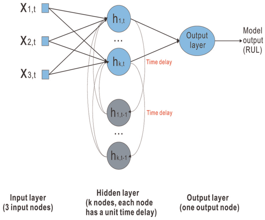
Architecture of a simple RNN.

ANNs can represent and build mappings from experience and historical measurements to predict RULs and adapt them to unobserved situations. The strong learning and generalization capabilities of ANNs render them suitable for modelling complex processes,¹⁰² particularly systems with nonlinear and time-varying dynamics.^106,108,109 In addition, ANNs are superior in capturing and presenting relationships between variables in high-dimensional data space, making them powerful tools for multidimensional interpolations,^{102,109–111} whereas RNNs are suitable for approximating dynamic dependencies.¹⁰⁷ These distinct characteristics make ANNs promising candidates for modelling degradation processes in rotating machinery.

Xu et al.¹¹² successfully employed RNNs, SVMs and DSR to estimate the RUL of an aircraft gas turbine. An echo state network (ESN), which is a variant of RNNs, was employed by Peng et al.¹¹³ to predict the RULs of engines using National Aeronautics and Space Administration (NASA) repository data. Their results indicate that the ESN significantly reduces the computing load of traditional RNNs. ANNs have also been used in combination with Kalman filters and extended Kalman filters^114,115 to predict failures in aircraft engines.

Although ANNs have been shown the superior power in addressing complex prognostic problems which have multivariate inputs, there are some limitations. For example, the majority of the ANN prognostic models aim to assume a single failure mode. Moreover, the models rely on a large amount of data for training. The prognostic accuracy is closely dependent on the quality of the training data.¹¹² Furthermore, ANNs allow for few explanatory insights into how the decisions are reached (also known as the black box problem), which has become concerning to modellers because causal relationships between model variables are essential for accurate descriptions of fault evolutions.¹¹⁶ Attempts to solve the black box problem can be found in Sussillo and Barak.¹¹⁷ Moreover, ANNs lack a systematic approach to determine the optimal structure and parameters of the network to be established.¹¹⁰ And in practice, the number and size of layers (especially hidden layers) are determined by testing a number of different combinations of numbers of layers and nodes, which is obviously time consuming. Thus, future studies should focus on establishing this systematic approach.

PHMs

Machine failures can be predicted by analysing either condition monitoring data or historical service lifetime data.^118,119 Developing appropriate prognostic models using a combination of condition-monitoring data and lifetime data would be useful. The PHM, proposed by Cox,¹²⁰ attempts to utilize both types of information for RUL prediction. The basic assumption of this method is that the failure rate of a machine depends on two factors: the baseline hazard rate and the effects of covariates (different condition monitoring variables). Hence, the hazard rate of a system at service time t can be written as $λ (t; z) = λ_{0} (t) \exp (β_{1} z_{1} + β_{2} z_{2} + \dots + β_{k} z_{k})$ , where $λ_{0} (t)$ denotes the baseline hazard function, which is determined by the system lifetime data, and $\exp (β_{1} z_{1} + β_{2} z_{2} + \dots + β_{k} z_{k})$ is the covariate function that describes how a number of monitoring variables influence health degradation. $z_{1}, z_{2}, \dots, z_{k}; β_{i}$ are unknown parameters to be determined that describes the effects of individual variable on system health.¹¹⁸ Applying PHMs requires that both the baseline hazard function $λ_{0} (t)$ and covariate function $\exp (z β)$ be identified. Methods that have been used to estimate the baseline function mainly consist of the maximum likelihood algorithm^120,121 and the Wald statistic.¹²² The covariate parameters can be determined by the so-called partial likelihood method, which is developed by Cox.¹²⁰ Subsequently, parameters are obtained by maximizing the partial likelihood, and key variables that are closely related to the system failure are retained and employed to estimate the system failure probability density.¹²³

PHMs have been applied to many complex problems regarding the failure prediction of rotating machinery. Jardine et al.¹²⁴ developed a PHM and employed it to estimate the RULs of aircraft engines and marine gas turbines. The baseline hazard function was assumed to be a Weibull distribution and was estimated using lifetime data. The levels of various metal particles, such as Fe, Cu and Mg, in the oil were used as the covariates in both cases. The influence of the condition-monitoring variables on the equipment RUL can be properly interpreted by this PHM. The authors also used the PHM to estimate the RUL and optimize maintenance decisions regarding haul truck wheel motors in Jardine et al.¹²² In this study, the key covariates related to failures were identified from 21 monitored oil analysis variables using the developed PHM. The results show that significant savings in maintenance costs could be achieved by optimizing the overhaul time as a function of lifetime data and oil analysis variables. However, the above models are based on the assumption that the system under study is subject to a single failure mode. In practice, most complex mechanical systems consist of multiple sub-systems with various failure modes.¹¹⁸ Therefore, a prognostic model that determines only one type of failure mode cannot properly estimate the overall system failure time. Recently, Zhang et al.¹¹⁸ proposed a mixed Weibull proportional hazard model (MWPHM) to assess the reliabilities of complex mechanical systems. In this model, the overall system failure probability density is determined by mixing the failure densities of various failure modes. The influences of multiple monitoring signals on different failure modes are integrated using the maximum likelihood estimation algorithm. Real data from a centrifugal water pump were combined with lifetime data to test the robustness of the model.

The main problem with using PHMs for failure prediction is that they require a large amount of lifetime data to determine the parameters of the baseline hazard function and the weighting of covariates.¹¹⁹ This requirement may limit the applications of PHMs because, in many cases, the amount of lifetime data may be insufficient for various reasons, including missing or non-existent records and transcription mistakes.¹²⁵ Another drawback of PHMs is that they depend on the failure thresholds chosen for RUL prediction. Thus, the threshold must be continuously updated when system maintenance is conducted.¹¹⁸ In addition, it is noteworthy that only the latest monitoring data rather than the whole observed history is used for RUL prediction, which may misdirect maintenance decision making.²⁰

Similarity-based models

Similarity-based prognostic models are essentially pattern matching approaches.¹²⁶ They are suitable for situations in which abundant run-to-failure data for a mechanical system are available.¹²⁷ The basic structure and working principle of such approaches is depicted in Figure 4.

Figure 4.

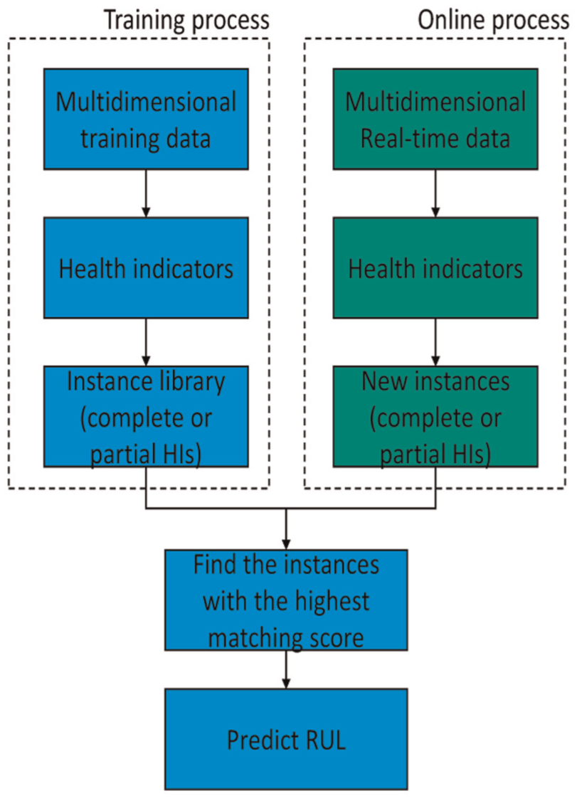
General framework of similarity-based prognostic models.

Multidimensional condition monitoring data collected from various operating conditions are first processed (e.g. noise reduction, feature extraction and multi-sensor data fusion) to produce a HI. This indicator represents the fault evolution using HI trajectories and is often a one-dimensional time series. Implementing the same processing operations to all training data sets, each multidimensional training series can be converted into a unique HI trajectory. Hence, a library of HI trajectories can be obtained during the training process. To predict the RUL using a new data set, the same processing operations are applied to the data to produce a new HI. Then, this new trajectory is compared with the library of HIs to determine which trajectory have the best matching scores (i.e. the most similar cases).¹²⁸ Those HIs with the highest similarities are subsequently used to predict the RUL.

Similarity-based methods differ from traditional prognostic models in that instead of fitting a curve for a system and extrapolating it, the sensory data are transformed into a HI trajectory and then compared to a library of HIs. The purpose of doing this is to match the new HI trajectory to a certain life period of a certain trajectory in the library. Then, the remnant life of the test component is calculated using the real life of the matching component subtracting the position of the matching life period.¹²⁷

The ability to accommodate multidimensional sensory measurements collected from various failure patterns makes similarity-based methods suitable for determining the prognostics of complex rotating machinery. Examples are given below to demonstrate how various similarity-based models have been used for RUL prediction.

Similarity model based on shapelet extraction

Malinowski et al.¹²⁸ developed a RUL prediction technique that employs the shapelet extraction process to extract failure patterns from multivariate data obtained from a turbofan engine simulation program: C-MAPSS. The RUL is calculated as the weighted sum of the failure patterns, which are highly corrected with the residual life.

Similarity model based on normalized cross correlation

Zhang et al.¹²⁹ applied a prognostic method based on the similarity of the phase space trajectory to the monitoring data collected from a pump with six distinct degradation modes.

Similarity model based on PCA and K-NN classifiers

Mosallam et al.¹³⁰ employed PCA and empirical mode decomposition (EMD) algorithms to construct HIs from turbofan engine deterioration data. Then, K-nearest neighbour (K-NN) classifiers were used to determine the most similar HIs for RUL prediction.

Similarity model based on belief functions

A method based on belief functions was proposed by Ramasso and colleagues.^131,132 These authors only matched the last points of the trajectories with tested ones because the last points are more likely to be closely related to the degradation state.

Similarity model based on linear regression and Euclidean distance measurement

Wang et al.¹²⁷ proposed a prognostic model in which the HI is obtained using linear regression. The best-matching instances are selected by examining the Euclidean distance between test and stored instances. This method has been applied to engine monitoring data to predict the RUL.

Similarity model based on support vector regression

Wang et al.¹³³ have improved upon the previous models by incorporating uncertainty information into the RUL estimation. Towards this end, they estimated HI degradation curves using RVM. Challenge data were employed to test the effectiveness of this method.

The advantage of similarity-based approaches is that they can deal with data collected from various failure modes and varying operating conditions. Furthermore, they can produce satisfactory and accurate predictions using abundant run-to-failure data. However, such data are commonly scarce in reality.¹²⁶ Additionally, many similarity-based prognostic techniques suffer from computational inefficiency in terms of sorting a large amount of training data.¹³¹ Hence, efforts should be made to extend these approaches to situations where limited training data are available and to reduce the computation complexity of such methods.

Summary of prognostic models of rotating machinery

In Table 1, the authors provide seven evaluation criteria that can be used to compare the prognostic techniques reviewed in this article. These criteria for each technique include the following:

Its ability to deal with nonlinear and non-stationary data.

Does this technique require large amounts of historical failure data?

Does this technique require a failure threshold?

Is this technique able to produce probabilistic results?

Is an analytical model a pre-requisite?

Requirements of historical condition monitoring data.

Prediction horizons (see column 2 of Table 2).

Table 1.

Comparison of different prognostic approaches.

Approach	Ability to deal with nonlinear and non-stationary data	Does this technique require large amounts of historical failure data?	Does this technique require a failure threshold?	Is this technique able to produce probabilistic results?	Is an analytical model a pre-requisite?	Requirements of historical condition monitoring data	Predict horizons
Distributed Kalman filter	No	No	Yes	Yes	Yes	Moderate data requirement	Able to generate multi-step ahead predictions
Support vector machine	Yes	No	Yes	No	No	Moderate data requirement	Predictions are made based on only current observations
Relevance vector machine	Yes	No	Yes	Yes	No	Moderate data requirement	Predictions are made based on only current observations
Particle filter	Yes	No	Yes	Yes	Yes	Moderate data requirement	Able to generate multi-step ahead predictions
Hidden Markov model and hidden semi-Markov model	Yes	No	Yes	Yes	No	Heavy historical condition monitoring data requirement	Able to generate multi-step ahead predictions
Stochastic filter	Yes	Yes	No	Yes	Yes	Heavy historical condition monitoring data requirement	Able to generate multi-step ahead predictions
Artificial neural network	Yes	No	Yes	No	No	Heavy historical condition monitoring data requirement	Able to generate multi-step ahead predictions
Proportional hazard model	No	Yes	Yes	No	No	Moderate data requirement	Predictions are made based on only current observations
Similarity-based model	Yes	No	Yes	No	No	Heavy historical condition monitoring data requirement	Able to generate multi-step ahead predictions

Table 2.

Applications of multidimensional prognostic models.

Rotating machine type	RUL prediction models
Gas turbine engines	SVM with Weibull function⁵⁷
	PSO-RBF-SVM⁶²
	Particle filter with PCA⁷⁹
	Particle filter with linear regression⁸¹
	Regularized particle filtering⁸²
	Particle filter with physical model⁷²
	HMM with ANN²
	Stochastic filter with PCA⁹⁷
	Stochastic filter with ICA⁹⁹
	Stochastic filter³⁸
	RNN, SVM and DSR¹¹²
	ESN¹¹³
	ANN with Kalman filters¹¹⁴
	ANN with extended Kalman filters¹¹⁵
	PHM with Weibull distribution¹²⁴
	Similarity model based on shapelet extraction¹²⁸
	Similarity model based on PCA and K-NN classifiers¹³⁰
	Similarity model based on belief functions^131,132
	Similarity model based on linear regression and Euclidean distance measurement¹²⁷
	Similarity model based on support vector regression¹³³
Pumps	HSMM⁹³
	AHSMM⁹⁴
	MWPHM¹¹⁸
	Similarity model based on normalized cross correlation¹²⁹
Diesel engines	Stochastic filter with PCA⁹⁸
Milling machines	DKF³⁰
	HMM⁸⁹
	HHMM⁹⁰
Haul truck wheel motors	PHM¹²²
Bearings	LSSVM with PCA⁶³
	Particle filter⁸⁰
	HMM⁹¹
	HSMM⁹⁵
	Stochastic filter with PCA¹⁰⁰
	Particle filter with adaptive FPT selection³⁹
	Particle filter with weighted minimum quantization error³⁷

RUL: remaining useful life; SVM: support vector machine; PSO: particle swarm optimization; RBF: radial-based function; PCA: principal component analysis; HMM: hidden Markov model; ANN: artificial neural network; ICA: independent component analysis; RNN: recurrent neural network; DSR: Dempster–Shafer regression; ESN: echo state network; PHM: proportional hazard model; K-NN: K-nearest neighbour; HSMM: hidden semi-Markov model; AHSMM: adaptive hidden semi-Markov model; MWPHM: Weibull proportional hazard model; DKF: distributed Kalman filter; HHMM: hierarchical hidden Markov model; LSSVM: least squares support vector machine; FPT: first predicting time.

Readers can use the listed criteria to compare different prognostic techniques according to practical needs.

Table 2 summarizes the applications of different RUL prediction models to various multi-sensor rotating machines and the machines common available data types. Furthermore, the reviewed articles (those appearing in Table 1) are classified based on the type of data employed in the article:

Simulated data collected from simulation programs, such as C-MAPSS;

Field data (real-world condition-monitoring data);

Data collected from experimental test rigs.

Figure 5 summarizes the types of data used in the studies reviewed.

Figure 5.

Type of data used in studies regarding various reviewed rotating machines.

According to the reviewed articles, the RUL estimate of gas turbine engines is the main application field. Moreover, about 50% of studies use simulation and experimental data for RUL analysis. This is because obtaining sufficient field data from operating machines is difficult and because inaccuracies may arise when applying these models to real-time data.

Conclusion

This article reviews multidimensional prognostic models for predicting the RULs of rotating machines. The prognostic models reviewed herein make predictions based on condition-monitoring information obtained from multiple sensors. Relevant theories are discussed, and the merits and limitations of the main prognostic model classes are detailed. Examples are given to explain how these approaches have been applied to predict RULs of multi-sensor rotating machinery. From the literature reviewed herein, a number of observations and suggestions can be made as follows:

The prognostic models reviewed herein can predict RULs accurately based on multi-source information. Compared to single-source prognostics, these models can provide more accurate results by considering the multi-source nature of the information. Therefore, they are particularly suitable for complex rotating systems because data from a single sensor cannot provide sufficient information to accurately analyse the degradation process.

In practice, the implementation of the models reviewed remains in the nascent stage, although a considerable number of studies have been performed based on simulated and experimental data. Therefore, efforts should be made to validate the effectiveness of these models using real-world data.

Although we may achieve more accurate prognostics using more sensor information, balancing the prediction accuracy and computational complexity remains challenging in practice. In addition, current sensor selection relies mainly on the developers’ observation of the raw condition-monitoring data (e.g. only variables exhibiting consistent trends or those acquired in components where a fault occurs are selected for further analysis). However, sometimes, the surrounding variables that are eliminated may also contain information relating to malfunctions because the system always operates as a whole entity. Therefore, future research should focus on developing (a) prognostic models with higher computational efficiencies and (b) sensor selection techniques that can automatically determine the optimum number of sensors for RUL prediction.

Many of the prognostic models reviewed provide probabilistic results to manage the estimation uncertainty caused by the stochastic nature of the degradation process. However, limited numbers of papers have studied the effects of performance deterioration in the multiple sensors. Hence, efforts should be made to quantify the influence of sensor degradation on uncertainties in RUL estimations.

In addition, future research should develop prognostic models that better adapt to continuously changing operating conditions (e.g. varying operating speed, input gas pressure and flow rate) during the degradation process.

Most of the techniques reviewed herein were originally designed for a signal failure mode occurring at a single defect point; therefore, future work should be focused on developing prognostic models that can be applied to multiple failure modes.

Most existing prognostic models consist of two phases: a learning phase, during which the analytical model is trained using run-to-failure data, and a testing phase, during which the trained model is employed to assess the state of the current system and to predict the systems RUL. However, few of these include a diagnostic model. Additional work is required to combine a multivariate diagnostic technique with the existing prognostic models, thereby allowing for online diagnosis and prognosis and real-time maintenance scheduling.

Footnotes

Academic Editor: Yonghui An

Declaration of conflicting interests

The author(s) declared no potential conflicts of interest with respect to the research, authorship, and/or publication of this article.

Funding

The author(s) disclosed receipt of the following financial support for the research, authorship, and/or publication of this article: This work was supported by London South Bank University.

References

Tran

Yang

BS.

An intelligent condition-based maintenance platform for rotating machinery. Expert Syst Appl 2012; 39: 2977–2988.

Giantomassi

Ferracuti

Benini

. Hidden Markov model for health estimation and prognosis of turbofan engines. In: Proceedings of the ASME 2011 international design engineering technical conferences and computers and information in engineering conference, Washington, DC, 28–31 August 2011, pp.681–689. New York: American Society of Mechanical Engineers.

Bevilacqua

Braglia

The analytic hierarchy process applied to maintenance strategy selection. Reliab Eng Syst Safe 2000; 70: 71–83.

Veldman

Klingenberg

Wortmann

Managing condition-based maintenance technology. J Qual Mainten Eng 2011; 17: 40–62.

Ruiz-Carcel

Lao

Cao

. Canonical variate analysis for performance degradation under faulty conditions. Control Eng Pract 2016; 54: 70–80.

Kan

Tan

ACC

Mathew

A review on prognostic techniques for non-stationary and non-linear rotating systems. Mech Syst Signal Pr 2015; 62: 1–20.

Heng

Zhang

Tan

ACC

. Rotating machinery prognostics: state of the art, challenges and opportunities. Mech Syst Signal Pr 2009; 23: 724–739.

Tobon-Mejia

Medjaher

Zerhouni

CNC machine tool’s wear diagnostic and prognostic by using dynamic Bayesian networks. Mech Syst Signal Pr 2012; 28: 167–182.

Tian

Zuo

SY.

Crack propagation assessment for spur gears using model-based analysis and simulation. J Intell Manuf 2012; 23: 239–253.

10.

Lee

Gear fatigue crack prognosis using embedded model, gear dynamic model and fracture mechanics. Mech Syst Signal Pr 2005; 19: 836–846.

11.

Chookah

Nuhi

Modarres

A probabilistic physics-of-failure model for prognostic health management of structures subject to pitting and corrosion-fatigue. Reliab Eng Syst Safe 2011; 96: 1601–1610.

12.

Marble

Morton

. Predicting the remaining life of propulsion system bearings. In: Proceedings of the IEEE aerospace conference, Big Sky, MT, 4–11 March 2006, pp.1–8. New York: IEEE.

13.

Patankar

Rao

MD.

Stochastic modeling of fatigue crack propagation by collective motion of dislocations. Int J Fatigue 2007; 29: 181–191.

14.

Kacprzynski

Sarlashkar

Roemer

. Predicting remaining life by fusing the physics of failure modeling with diagnostics. JOM: J Min Met Mat S 2004; 56: 29–35.

15.

Tran

. Machine condition prognosis using multi-step ahead prediction and neuro-fuzzy systems. In: Proceedings of the international symposium on advanced mechanical and power engineering, Busan, Korea, pp.1–6, http://eprints.hud.ac.uk/16568/

16.

Huang

ZG.

Remaining useful life prediction for a hidden wiener process with an adaptive drift. IEEE T Reliab 2013; 64: 1–14.

17.

Peng

Dong

A prognosis method using age-dependent hidden semi-Markov model for equipment health prediction. Mech Syst Signal Pr 2011; 25: 237–252.

18.

Zio

Di Maio

Stasi

A data-driven approach for predicting failure scenarios in nuclear systems. Ann Nucl Energy 2010; 37: 482–491.

19.

Goode

Moore

Roylance

BJ.

Plant machinery working life prediction method utilizing reliability and condition-monitoring data. Proc IMechE, Part E: J Process Mechanical Engineering 2000; 214: 109–122.

20.

Wang

Christer

AH.

Towards a general condition based maintenance model for a stochastic dynamic system. J Oper Res Soc 2000; 51: 145–155.

21.

Lee

Zhao

. Prognostics and health management design for rotary machinery systems – reviews, methodology and applications. Mech Syst Signal Pr 2014; 42: 314–334.

22.

Wang

. Remaining useful life estimation – a review on the statistical data driven approaches. Eur J Oper Res 2011; 213: 1–14.

23.

Sikorska

Hodkiewicz

Prognostic modelling options for remaining useful life estimation by industry. Mech Syst Signal Pr 2011; 25: 1803–1836.

24.

Zhang

GF.

Optimum sensor localization/selection in a diagnostic/prognostic architecture. PhD Thesis, Georgia Institute of Technology, Atlanta, GA, 2005.

25.

Padula

Kincaid

RK.

Optimization strategies for sensor and actuator placement. Technical report NASA/TM-1999-209126, April 1999. Hampton, VA: NASA.

26.

Jiang

. Optimal sensor location in closed-loop control systems for fault detection and isolation. In: Proceedings of the American control conference, Chicago, IL, 28–30 June 2000, pp.1195–1199. New York: IEEE.

27.

Raghuraj

Bhushan

Rengaswamy

Locating sensors in complex chemical plants based on fault diagnostic observability criteria. AIChE J 1999; 45: 310–322.

28.

Wang

Song

Wang

Statistical process monitoring using improved PCA with optimized sensor locations. J Process Contr 2002; 12: 735–744.

29.

Yang

Chen

Monte Carlo methods for reliability evaluation of linear sensor systems. IEEE T Reliab 2011; 60: 305–314.

30.

Wei

Chen

Zhou

DH.

Multi-sensor information based remaining useful life prediction with anticipated performance. IEEE T Reliab 2013; 62: 183–198.

31.

Sharifi

Langari

Nonlinear sensor fault diagnosis using mixture of probabilistic PCA models. Mech Syst Signal Pr 2017; 85: 638–650.

32.

Chen

. A statistical training data cleaning strategy for the PCA-based chiller sensor fault detection, diagnosis and data reconstruction method. Energ Buildings 2016; 112: 270–278.

33.

Liu

Peng

Liu

FESeR: a data-driven framework to enhance sensor reliability for the system condition monitoring. Microelectron Reliab 2016; 64: 681–687.

34.

Safizadeh

Latifi

SK.

Using multi-sensor data fusion for vibration fault diagnosis of rolling element bearings by accelerometer and load cell. Inform Fusion 2014; 18: 1–8.

35.

Kolarik

WJ.

Multivariate performance reliability prediction in real-time. Reliab Eng Syst Safe 2001; 72: 39–45.

36.

Caesarendra

Widodo

Thom

. Combined probability approach and indirect data-driven method for bearing degradation prognostics. IEEE T Reliab 2011; 60: 14–20.

37.

Lei

Gontarz

. A model-based method for remaining useful life prediction of machinery. IEEE T Reliab 2016; 65: 1314–1326.

38.

Wei

Chen

Zhou

DH.

Remaining useful life prediction using a stochastic filtering model with multi-sensor information fusion. In: Proceedings of the 2011 prognostics and system health management conference, Shenzhen, China, 24–25 May 2011, pp.1–6. New York: IEEE.

39.

Lei

. An improved exponential model for predicting the remaining useful life of lithium-ion batteries. IEEE T Ind Electron 2015; 62: 7762–7773.

40.

Jiang

Huang

Zhu

. Canonical variate analysis-based contributions for fault identification. J Process Contr 2015; 26: 17–25.

41.

Jiang

Zhu

Huang

. Canonical variate analysis-based monitoring of process correlation structure using causal feature representation. J Process Contr 2015; 32: 109–116.

42.

Yunus

MYM

Zhang

. Multivariate process monitoring using classical multidimensional scaling and procrustes analysis. In: Proceedings of the 9th international symposium on dynamics and control of process systems, Leuven, 5–7 July 2010, vol. 9, pp.165–170. Elsevier Ltd.

43.

Alkaya

Eker

Variance sensitive adaptive threshold-based PCA method for fault detection with experimental application. ISA T 2011; 50: 287–302.

44.

Spanos

Murray

RM.

Approximate distributed Kalman filtering in sensor networks with quantifiable performance. In: Proceedings of the 4th international symposium on information processing in sensor networks, Boise, ID, 15 April 2005, pp.133–139. Piscataway, NJ: IEEE Press.

45.

Speyer

JL.

Computation and transmission requirements for a decentralized linear-quadratic-Gaussian control problem. IEEE T Automat Contr 1979; 24: 266–269.

46.

Cattivelli

Sayed

AH.

Diffusion strategies for distributed Kalman filtering and smoothing. IEEE T Automat Contr 2010; 55: 2069–2084.

47.

Durrant-Whyte

Berg

TM.

General decentralized Kalman filters. In: Proceedings of the 1994 American control conference, Baltimore, MD, 29 June–1 July 1994, vol. 2, pp.4–5. New York: IEEE.

48.

Grime

Durrant-Whyte

HF.

Data fusion in decentralized sensor networks. Control Eng Pract 1994; 2: 849–863.

49.

Lendek

Babuška

Schutter

. Distributed Kalman filtering for multiagent systems. In: Proceedings of the European control conference 2007 (ECC’07), Kos, 2–5 July 2007, vol. 19, pp.2193–2200. New York: IEEE.

50.

Zhu

You

Zhao

. The optimality for the distributed Kalman filtering fusion with feedback. Automatica 2001; 37: 1489–1493.

51.

Olfati-Saber

. Distributed Kalman filtering for sensor networks. In: Proceedings of the IEEE conference on decision and control, New Orleans, LA, 12–14 December 2007, pp.5492–5498. New York: IEEE.

52.

Boser

Guyon

Vapnik

. A training algorithm for optimal margin classifiers. In: Proceedings of the 5th annual ACM workshop on computational learning theory, Pittsburgh, PA, 27–29 July 1992, pp.144–152. New York: ACM.

53.

Drucker

Kaufman

Support vector regression machines. Neural Inform Process Syst 1997; 9: 155–161.

54.

Delgado

Garcia

Ortega

. Multidimensional intelligent diagnosis system based on support vector machine classifier. In: Proceedings of the 2011 IEEE international symposium on industrial electronics, Gdansk, 27–30 June 2011, pp.2124–2131. New York: IEEE.

55.

Saha

Goebel

Christophersen

Comparison of prognostic algorithms for estimating remaining useful life of batteries. T I Meas Control 2009; 31: 293–308.

56.

Huang

Wang

. Support vector machine based estimation of remaining useful life: current research status and future trends. J Mech Sci Technol 2015; 29: 151–163.

57.

Louen

Ding

Kandler

. A new framework for remaining useful life estimation using support vector machine classifier. In: Proceedings of the 2013 conference on control and fault-tolerant systems (SysTol), Nice, 9–11 October 2013, pp.1–6. New York: IEEE.

58.

Karacali

Ramanath

Snyder

WE.

A comparative analysis of structural risk minimization by support vector machines and nearest neighbor rule. Pattern Recogn Lett 2004; 25: 63–71.

59.

Zhang

Liu

Luo

. Review of remaining useful life prediction using support vector machine for engineering assets. In: Proceedings of the 2013 international conference on quality, reliability, risk, maintenance, and safety engineering (QR2MSE), Chengdu, China, 15–18 July 2013, pp.1793–1799. New York: IEEE.

60.

Niu

Yang

BS.

Intelligent condition monitoring and prognostics system based on data-fusion strategy. Expert Syst Appl 2010; 37: 8831–8840.

61.

Wang

TY.

Trajectory similarity based prediction for remaining useful life estimation. PhD Thesis, University of Cincinnati, Cincinnati, OH, 2010.

62.

Garcia Nieto

Garcia-Gonzalo

Sanchez Lasheras

. Hybrid PSO–SVM-based method for forecasting of the remaining useful life for aircraft engines and evaluation of its reliability. Reliab Eng Syst Safe 2015; 138: 219–231.

63.

Chen

Hong

. Degradation trend estimation of slewing bearing based on LSSVM model. Mech Syst Signal Pr 2016; 76–77: 353–366.

64.

Qian

Wang

GG.

Fault prognostic based on hybrid method of state judgment and regression. Adv Mech Eng 2013; 2013: 149562.

65.

Tipping

Sparse Bayesian learning and the relevance vector mach. J Mach Learn Res 2001; 1: 211–244.

66.

Bolic

Djuric

PM.

Resampling methods for particle filtering: classification, implementation, and strategies. IEEE Signal Proc Mag 2015; 32: 70–86.

67.

Arulampalam

Maskell

Gordon

. A tutorial on particle filters for online nonlinear/non-Gaussian Bayesian tracking. IEEE T Signal Proces 2002; 50: 174–188.

68.

Choi

Kim

NH.

Prognostics 101: a tutorial for particle filter-based prognostics algorithm using Matlab. Reliab Eng Syst Safe 2013; 115: 161–169.

69.

Fan

Yung

Pecht

Predicting long-term lumen maintenance life of LED light sources using a particle filter-based prognostic approach. Expert Syst Appl 2015; 42: 2411–2420.

70.

Jouin

Gouriveau

Hissel

. Particle filter-based prognostics: review, discussion and perspectives. Mech Syst Signal Pr 2015; 73: 2–31.

71.

Baraldi

Di Maio

. A particle filtering and kernel smoothing-based approach for new design component prognostics. Reliab Eng Syst Safe 2014; 134: 19–31.

72.

Baraldi

Cadini

Mangili

. Prognostics under different available information. Chem Eng Trans 2013; 33: 163–168.

73.

Chen

Tang

. A novel PF-LSSVR-based framework for failure prognosis of nonlinear systems with time-varying parameters. Chinese J Aeronaut 2012; 25: 715–724.

74.

Liu

Wang

. A data-model-fusion prognostic framework for dynamic system state forecasting. Eng Appl Artif Intel 2012; 25: 814–823.

75.

Orchard

Vachtsevanos

. A particle filtering framework for failure prognosis. In: Proceedings of the WTC2005 world tribology congress III, Washington, DC, 12–16 September 2005, pp.1–2. New York: ASME.

76.

Saha

Goebel

Modeling Li-ion battery capacity depletion in a particle filtering framework. In: Proceedings of the annual conference of the prognostics and health management society, San Diego, CA, 27 September–1 October 2009, pp.2909–2924. phmsociety.

77.

Borges

Cerdeira

Kawakami

. Particle filter prognostic applied in landing gear retraction. In: Proceedings of the annual conference of the prognostics and health management society, New Orleans, LA, 14–17 October 2013, pp.1–8. phmsociety.

78.

Carpenter

Clifford

Fearnhead

Improved particle filter for nonlinear problems. IEEE Proc: Radar Sonar Navig 1999; 146: 2–7.

79.

Wang

A prognosis model for wear prediction based on oil-based monitoring. J Oper Res Soc 2007; 58: 887–893.

80.

Butler

O’Connor

Farren

. A feasibility study into prognostics for the main bearing of a wind turbine. In: Proceedings of the IEEE international conference on control applications, Dubrovnik, 3–5 October 2012, pp.1092–1097. New York: IEEE.

81.

Sun

Zuo

Wang

. Application of a state space modeling technique to system prognostics based on a health index for condition-based maintenance. Mech Syst Signal Pr 2012; 28: 585–596.

82.

Wang

Gao

RX.

Particle filtering-based system degradation prediction applied to jet engines. In: Proceedings of the annual conference of the prognostics and health management society, Fort Worth, TX, 29 September–2 October 2014, pp.1–6. phmsociety.

83.

Rabiner

LR.

A tutorial on hidden Markov models and selected applications in speech recognition. P IEEE 1989; 77: 257–286.

84.

Schuster-Böckler

Bateman

An introduction to hidden Markov models. IEEE ASSP Mag 1986; 86: 4–16.

85.

Viterbi

AJ.

Error bounds for convolutional codes and an asymptotically optimum decoding algorithm. IEEE T Inform Theory 1967; 13: 260–269.

86.

Bunks

Mccarthy

Al-Ani

Condition-based maintenance of machines using hidden Markov models. Mech Syst Signal Pr 2000; 14: 597–612.

87.

Baruah

Chinnam

RB.

HMMs for diagnostics and prognostics in machining processes. Int J Prod Res 2005; 43: 1275–1293.

88.

Chinnam

Baruah

Autonomous diagnostics and prognostics through competitive learning driven HMM-based clustering. In: Proceedings of the international joint conference on neural networks, Portland, OR, 20–24 July 2003, vol. 4, pp.2466–2471. New York: IEEE.

89.

Camci

Chinnam

RB.

Health-state estimation and prognostics in machining processes. IEEE T Autom Sci Eng 2010; 7: 581–597.

90.

Fine

The hierarchical hidden Markov model: analysis and applications. Mach Learn 1998; 32: 41–62.

91.

Soualhi

Clerc

Razik

. Hidden Markov models for the prediction of impending faults. IEEE T Ind Electron 2016; 63: 3271–3281.

92.

Srinivasan

Parlikad

AKN

. Semi-Markov decision process with partial information for maintenance decisions. IEEE T Reliab 2014; 63: 891–898.

93.

Dong

Hidden semi-Markov model-based methodology for multi-sensor equipment health diagnosis and prognosis. Eur J Oper Res 2007; 178: 858–878.

94.

Liu

Dong

. A novel method using adaptive hidden semi-Markov model for multi-sensor monitoring equipment health prognosis. Mech Syst Signal Pr 2015; 64–65: 217–232.

95.

Chen

Yang

. Fault prognosis of complex mechanical systems based on multi-sensor mixtured hidden semi-Markov models. Proc IMechE, Part C: J Mechanical Engineering Science 2012; 227: 1853–1863.

96.

Geramifard

Zhou

. A physically segmented hidden Markov model approach for continuous tool condition monitoring: diagnostics and prognostics. IEEE T Ind Inform 2012; 8: 964–973.

97.

Wang

Zhang

WJ.

A model to predict the residual life of aircraft engines based upon oil analysis data. Nav Res Log 2005; 52: 276–284.

98.

Wang

Hussin

Jefferis

A case study of condition based maintenance modelling based upon the oil analysis data of marine diesel engines using stochastic filtering. Int J Prod Econ 2012; 136: 84–92.

99.

Wang

Hussin

Plant residual time modelling based on observed variables in oil samples. J Oper Res Soc 2009; 60: 789–796.

100.

Wang

WB.

A two-stage prognosis model in condition based maintenance. Eur J Oper Res 2007; 182: 1177–1187.

101.

Rafiq

Bugmann

Easterbrook

DJ.

Neural network design for engineering applications. Comput Struct 2001; 79: 1541–1552.

102.

Rodriguez

El Hamzaoui

Hernandez

. The use of artificial neural network (ANN) for modeling the useful life of the failure assessment in blades of steam turbines. Eng Fail Anal 2013; 35: 562–575.

103.

Atiya

El-Shoura

Shaheen

. A comparison between neural-network forecasting techniques – case study: river flow forecasting. IEEE T Neural Networ 1999; 10: 402–409.

104.

Gencay

Liu

Nonlinear modelling and prediction with feedforward and recurrent networks. Physica D 1997; 108: 119–134.

105.

Mukherjee

Routroy

Comparing the performance of neural networks developed by using Levenberg–Marquardt and Quasi-Newton with the gradient descent algorithm for modelling a multiple response grinding process. Expert Syst Appl 2012; 39: 2397–2407.

106.

Ahmadzadeh

Lundberg

Remaining useful life prediction of grinding mill liners using an artificial neural network. Miner Eng 2013; 53: 1–8.

107.

Liu

Djurdjanovic

. Similarity based method for manufacturing process performance prediction and diagnosis. Comput Ind 2007; 58: 558–566.

108.

Senjyu

Takara

Uezato

. One-hour-ahead load forecasting using neural network. IEEE T Power Syst 2002; 17: 113–118.

109.

Zhang

Ganesan

Multivariable trend analysis using neural networks for intelligent diagnostics of rotating machinery. J Eng Gas Turb Power 1997; 119: 378–384.

110.

Zhang

Wang

Fault diagnosis and prognosis using wavelet packet decomposition, Fourier transform and artificial neural network. J Intell Manuf 2012; 24: 1213–1227.

111.

Wang

SH.

Application of self-organising maps for data mining with incomplete data sets. Neural Comput Appl 2003; 12: 42–48.

112.

Wang

PHM-oriented integrated fusion prognostics for aircraft engines based on sensor data. IEEE Sens J 2014; 14: 1124–1132.

113.

Peng

Wang

. A modified echo state network based remaining useful life estimation approach. In: Proceedings of the 2012 IEEE conference on prognostics and health management (PHM), Denver, CO, 18–21 June 2012, pp.1–7. New York: IEEE.

114.

Peel

. Data driven prognostics using a Kalman filter ensemble of neural network models. In: Proceedings of the international conference on prognostics and health managements, Denver, CO, 6–9 October 2008, pp.1–6. New York: IEEE.

115.

Heimes

. Recurrent neural networks for remaining useful life estimation. In: Proceedings of the international conference on prognostics and health management, Denver, CO, 6–9 October 2008, pp.1–6. New York: IEEE.

116.

Olden

Jackson

DA.

Illuminating the ‘black box’: a randomization approach for understanding variable contributions in artificial neural networks. Ecol Model 2002; 154: 135–150.

117.

Sussillo

Barak

Opening the black box: low-dimensional dynamics in high-dimensional recurrent neural networks. Neural Comput 2013; 25: 626–649.

118.

Zhang

Hua

GH.

A mixture Weibull proportional hazard model for mechanical system failure prediction utilising lifetime and monitoring data. Mech Syst Signal Pr 2014; 43: 103–112.

119.

Sun

Mathew

. Mechanical systems hazard estimation using condition monitoring. Mech Syst Signal Pr 2006; 20: 1189–1201.

120.

Cox

DR.

Regression models and life-tables. J Roy Stat Soc B Met 1972; 34: 187–220.

121.

Tran

Thom Pham

Yang

. Machine performance degradation assessment and remaining useful life prediction using proportional hazard model and support vector machine. Mech Syst Signal Pr 2012; 32: 320–330.

122.

Jardine

AKS

Banjevic

Wiseman

. Optimizing a mine haul truck wheel motors’ condition monitoring program: use of proportional hazards modeling. J Qual Mainten Eng 2001; 7: 286–302.

123.

Bendell

Proportional hazards modelling in reliability assessment. Reliab Eng 1985; 11: 175–183.

124.

Jardine

AKS

Anderson

Mann

DS.

Application of the Weibull proportional hazards model to aircraft and marine engine failure data. Qual Reliab Eng Int 1986; 3: 77–82.

125.

Manuel

Carlos

Pereira

. Data management for CBM optimization. J Qual Mainten Eng 2008; 12: 37–51.

126.

Liao

Köttig

Review of hybrid prognostics approaches for remaining useful life prediction of engineered systems, and an application to battery life prediction. IEEE T Reliab 2014; 63: 191–207.

127.

Wang

Siegel

. A similarity based prognostic approach for remaining useful life estimation of engineered systems. In: Proceedings of the international conference on prognostics and heath management, Denver, CO, 8–10 July 2014, pp.4–9. phmsociety.

128.

Malinowski

Chebel-Morello

Zerhouni

Remaining useful life estimation based on discriminating shapelet extraction. Reliab Eng Syst Safe 2015; 142: 279–288.

129.

Zhang

Tse

PWT

Wan

. Remaining useful life estimation for mechanical systems based on similarity of phase space trajectory. Expert Syst Appl 2015; 42: 2353–2360.

130.

Mosallam

Medjaher

Zerhouni

Data-driven prognostic method based on Bayesian approaches for direct remaining useful life prediction. J Intell Manuf 2016; 27: 1037–1048.

131.

Ramasso

Rombaut

Zerhouni

Joint prediction of continuous and discrete states in time-series based on belief functions. IEEE T Cybern 2013; 43: 37–50.

132.

Ramasso

Gouriveau

Remaining useful life estimation by classification of predictions based on a neuro-fuzzy system and theory of belief functions. IEEE T Reliab 2014; 63: 555–566.

133.

Wang

Youn

A generic probabilistic framework for structural health prognostics and uncertainty management. Mech Syst Signal Pr 2012; 28: 622–637.

Multidimensional prognostics for rotating machinery: A review

Abstract

Keywords

Introduction

Definition of multidimensional prognostics

Discussion on multidimensional prognostic models

Kalman filter–based models

SVM and RVM

SVM

RVM

Particle filter

HMM and HSMM

HMM

HSMM

Stochastic filter

ANN-based models

PHMs

Similarity-based models

Similarity model based on shapelet extraction

Similarity model based on normalized cross correlation

Similarity model based on PCA and K-NN classifiers

Similarity model based on belief functions

Similarity model based on linear regression and Euclidean distance measurement

Similarity model based on support vector regression

Summary of prognostic models of rotating machinery

Conclusion

Footnotes

Declaration of conflicting interests

Funding

References