
Abstract
A canned nuclear coolant pump is used in an advanced third-generation pressurized water reactor. Impeller is a key component of a canned nuclear coolant pump. Usually, the blade is installed between the hub and the shroud as an entire part. The blade is divided into two parts and is staggered in the circumferential direction is an approach of blade design. To understand the effects of staggered blades on a canned nuclear coolant pump, this article numerically investigated different types of staggering. The validity of the numerical simulation was confirmed by comparing the numerical and experimental results. The performance change of a canned nuclear coolant pump with staggered blades was acquired. Hydraulic performance curves, axial force curves, static pressure distributions at the impeller outlet, and static pressure pulsations were performed to investigate the performance changes caused by the staggered blades. The results show that the staggered blade has an important influence on the performance of canned nuclear coolant pumps. A staggered blade does not improve hydraulic performance but does improve the axial force and pressure pulsation. Specifically, the staggered blades can significantly reduce the pressure pulsation amplitude on the impeller pass frequency.
Keywords
Introduction
The reactor coolant pump that is used to circulate coolant between the reactor and the steam generator is key equipment in a nuclear power station. The reactor coolant pump used in an advanced third-generation pressurized water reactor is a canned pump, called a canned nuclear coolant pump. The hydraulic components are located on the canned motor and are composed of a suction adapter, an impeller, a radial diffuser, and an annular discharge case. A sketch of the structure is shown in Figure 1. The canned nuclear coolant pump for a currently planned 1400-MW power station unit (CAP1400) needs hydraulic components to produce the following data at the rated operating point: Q = 21,642 m3/h, H = 111 m, and n = 1485 r/min. The impeller type is closed, and the specific speed is approximately 105. High efficiency, low power consumption, low axial force, and low pressure pulsation are significant hydraulic performance features that are demanded of hydraulic components. Thus, it was decided to build a hydraulic model 1 (on a scale of 1:2.5) to study the model pump rated operating data: Q = 1385 m3/h, H = 18 m, and n = 1485 r/min.

Canned nuclear coolant pump hydraulic components.
The impeller design is the key to the canned nuclear coolant pump performance. Usually, the design of the impeller comprises the following steps:2,3 (1) calculate the main geometric parameters based on the similarity coefficient and statistical data and then draw the meridian section of the impeller, (2) select the number of blades, (3) calculate the blade thickness based on structural strength requirements, and (4) design the central profile of the blade. Usually, the impeller blade is installed between the hub and the shroud in the pump and compressor as an entire part, 4 but there are other different blade forms such as splitter blades5–7 and tandem blades.8–10 Splitter blades are transformed in the blade-to-blade direction, and tandem blades are transformed in the streamline direction similar to the series approach. Thus, a staggered blade is transformed in the span direction, similar to the parallel approach. Staggered blades have been used in fans for noise reduction.11,12
In this article, different staggered blade impellers will be investigated to show the influence of staggered blades on a canned nuclear coolant pump. Based on numerical calculations of a model pump, the changes and different performances in hydraulic performance curves, axial force curves, static pressure distributions at the impeller outlet, and static pressure pulsations were investigated.
Geometry description
The entire blade is divided into two parts by a rib from the leading edge to the trail edge so that the two parts can be staggered from each other in the circumferential direction, somewhat similar to some double-suction pumps.13,14 The blade design is shown in Figures 2 and 3. There are three different ways of transforming the meridian plane according to different flow rates from the hub to the shroud, as shown in Figure 3. A third of the rated flow Qr near the hub side is indicated with 1/3, the same rated flow Qr for both sides is indicated with 1/2, and a third of the rated flow Qr near the shroud side is indicated with 2/3. Additionally, there are three different staggered angles between the hub side and the shroud side along the circumference rotation direction, as shown in Figure 4: 18°, 36°, and 54°. Thus, there are nine different forms of staggered blades, but only five forms can describe the effects of staggered blades: 1/2–18, 1/2–36, 1/2–54, 1/3–36, and 2/3–36; these are expressed as case 1, case 2, case 3, case 4, and case 5, respectively. We choose a 1/2–36 staggered blade to compare the differences between an original blade and a staggered blade. Different flows can be used with the same staggered angle to show the influence of the flow on the model pump; also, different staggered angles can be used with the same flows to show the influence of the staggered angle on the model pump. In this study, the number of original impeller blades is 5, and the number of diffuser vanes is 13. No other static parts are changed.
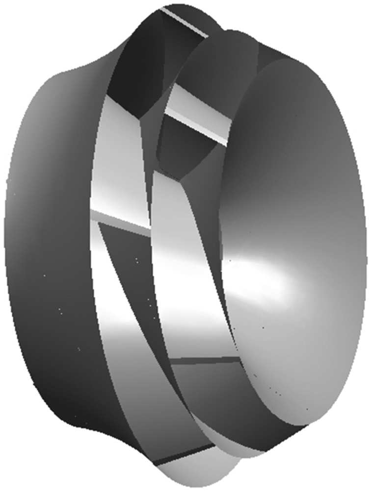
Impeller with staggered blades.

Staggered with different flow rates.

Staggered with different staggered angles.
Numerical calculation setup
Calculation models and mesh
The calculation domain was created based on the model pump machine; the entire flow domain in the computational fluid dynamics (CFD) model consists of the inlet, impeller, diffuser, case, chamber, and gaps. To obtain a relatively stable inlet and outlet, the inlet section was extended to three times the impeller inlet diameter, and the outlet section was extended to five times the impeller outlet diameter. Specifically, the gap width was doubled according to the real model pump machine. The calculation flow domain is shown in Figure 5.

Divided 3D model domains.
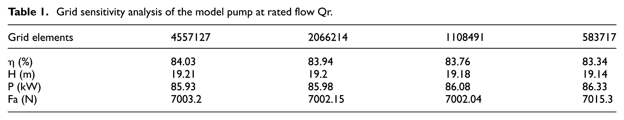
TurboGrid was used to generate a structured grid for the impeller. The value of y+ near the boundary wall was set to 100; 15 the total grid element number was approximately 1.0 × 10⁶. In comparison, the mesh number for different blades was approximately the same. The mesh of the impeller is shown in Figure 6. The Integrated Computer Engineering and Manufacturing code for Computational Fluid Dynamics (ICEMCFD) was used to generate an unstructured grid for other static components, and the total grid element number was approximately 2.0 × 10⁶. 16 Table 1 shows the results of the grid sensitivity analysis. The grid element number in Table 1 is an unstructured grid for other static components; the structured grid number of impellers was kept constant. It can be seen that the values experience only a slight change, which indicates that the simulation results are becoming stable.

Structured mesh of the impeller.
Grid sensitivity analysis of the model pump at rated flow Qr.
Computational methods and setup
The ANSYS-CFX was selected for the solution of the fully three-dimensional (3D) incompressible Navier–Stokes equations. The turbulence model that was selected was k–ε mode with the nonslip wall condition. Second-order upwind discretization was used for the convection term. The convergence criterion was 10e−5, which is used in the pump performance calculation. The fluid that was selected was ideal water at 25°C. The boundary condition for the inlet was static pressure and for the outlet was mass flow, which is said to be stable, converges quickly, and is used often.17,18
In the steady calculation state, the simulation used the multireference frame technique, in which the impeller is situated in the rotating reference frame, and other static components are in the fixed reference frame. They are related to each other through the interface “stage.” In the unsteady calculation state, the impeller and static components are related to each other through the interface “transient rotor stator.” The steady calculation results were the initial condition for the unsteady calculation. The time step Δt = 2.2447 × 10⁻⁴ s, which is said to be accurate;19–21 all 180 steps are in one rotating circle, calculating 15 circles in total, which is said to be accurate. 22
Comparison of the test and numerical calculation
A set of hydraulic components for the CAP1400 canned nuclear pump model was designed before using the numerical setup and calculation described above to predict performance. The model pump test was carried out at the National Industrial Pump Quality Supervision Test Center in Shenyang, China. Figure 7 shows the model pump test device. The comparison of the numerical CFD results with the test results is described in Figure 8. Because the CFD simulation ignored the wall roughness, mechanical loss, and volume loss, it can be seen that the numerical CFD calculated values were greater than the test, while the trend of the curves was the same. Thus, the numerical setup and calculation described above can be used to predict pump performance with acceptable accuracy.
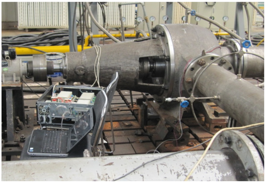
The 1:2.5 model pump test.

Numerical calculation and test results: (a) efficiency with different Q, (b) head with different Q, (c) power with different Q, and (d) axial force with different Q.
Steady CFD results and analysis
The efficiency, head, power, and axial force of the model pump with different staggered blades were investigated by CFD calculations. The canned nuclear coolant pump always works near the rated operating point Qr at rated speed because of the variable starting and stopping frequency that is used by the canned motor. So, the CFD calculation was from 0.85Qr to 1.15Qr. The Q–η curve, Q–H curve, Q–P curve, and Q–Fa curve of different staggered blades were calculated. Q (m3/h) is the flow rate, η (%) is the efficiency, H (m) is the head, P (kW) is the power, and Fa (N) is the axial force. Then, three different comparisons were used for illustration.
Staggered blade and original blade
First, staggered blade case 2 and the original blade were discussed. The characteristic curves of a canned nuclear model pump are shown in Figure 9(a)–(c). Because of the impact and friction losses of the rib and the mixed loss at the impeller outlet, it can be seen that the efficiency and head curves of staggered blades are decreased relative to the original blade, and that the power curve is increased. The maximum efficiency point of the staggered blade moves to large flow; the efficiency difference is smaller in 1.0Qr–1.15Qr and greater in 0.85Qr–1.0Qr. The slope dH/dQ is decreased gradually from 1.15Qr to 0.85Qr, and the head difference increased gradually. The maximum power point is not changed, and the power is increased gradually from 1.15Qr to 0.85Qr. Thus, staggered blade case 2 reduces the efficiency and the head slightly.

Numerical characteristic curves of the staggered and original blades: (a) efficiency Q–η curve, (b) head Q–H curve, and (c) power Q–P curve.
The differences in axial forces with staggered blade case 2 and the original blade are shown in Figure 10. The difference between the two axial forces acting on the impeller hub and shroud is shown in Figure 10(a). The difference between the momentum axial force and the total axial force is shown in Figure 10(b); the upper part is the total axial force. It can be seen that the axial force curves of the staggered blade are decreased relative to the original blade. The axial force slope of the staggered blade is decreased from 0.95Qr to 0.85Qr in Figure 10(a), and the axial force is greater than the original blade at 0.85Qr. The slope of the momentum axial force is approximately the same, and the total axial forces are increasingly close to each other from 0.95Qr to 0.85Qr, as shown in Figure 10(b). Thus, staggered blade case 2 reduces the axial force slightly.

Numerical axial force of the staggered and original blades: (a) difference between the hub and shroud and (b) momentum axial force and total axial force.
Different staggered angles with the same flow rate
Three different staggered angles were discussed: case 1, case 2, and case 3. The characteristic curves of a canned nuclear model pump are shown in Figure 11(a)–(c). The numerical hydraulic performance results of different staggered angles are shown in Table 2. It can be seen that the staggered angle has almost no influence on pump performance.
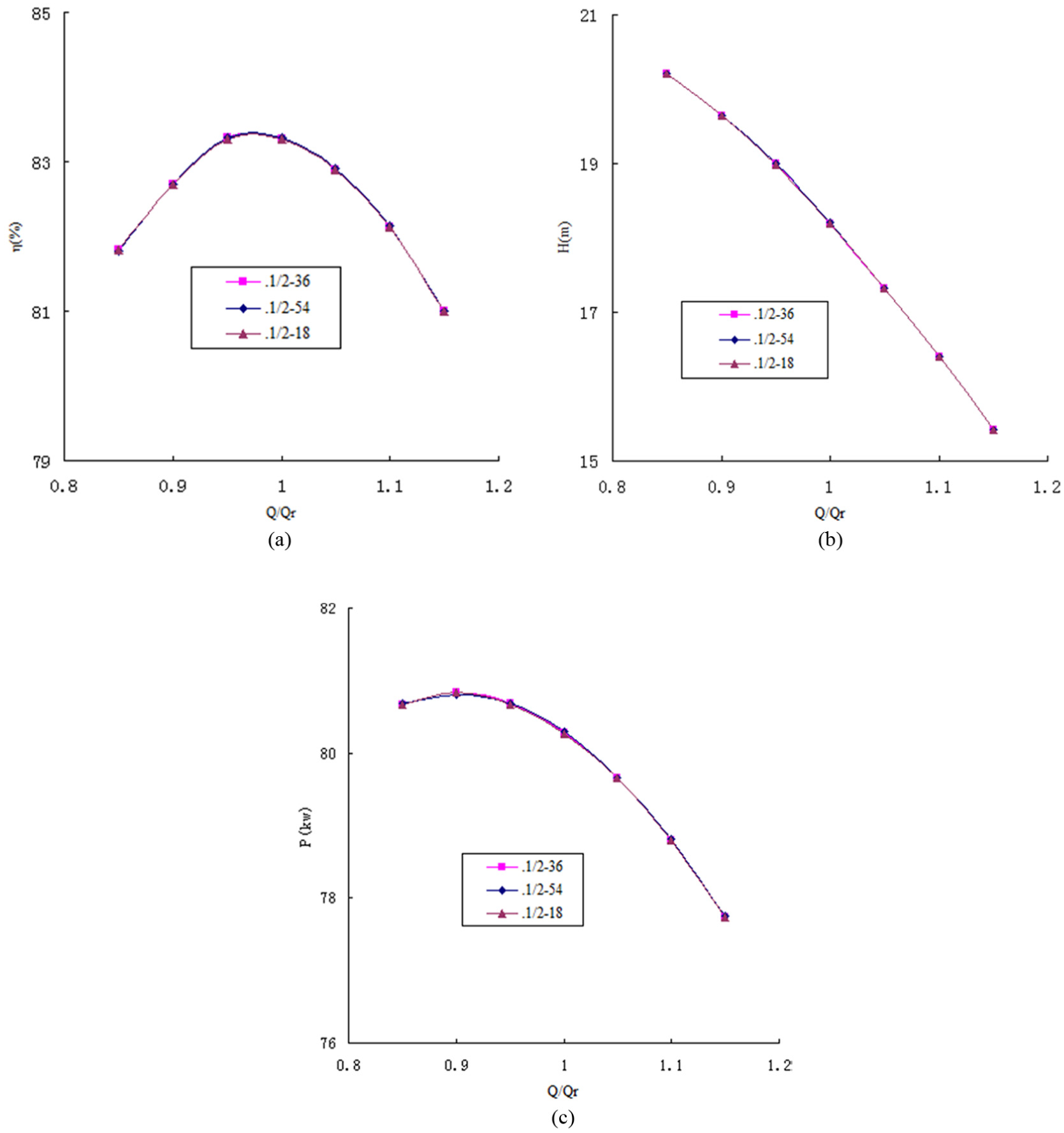
Numerical characteristic curves of different staggered angles: (a) efficiency Q–η curve, (b) head Q–H curve, and (c) power Q–P curve.
Numerical hydraulic performance results of different staggered angles.

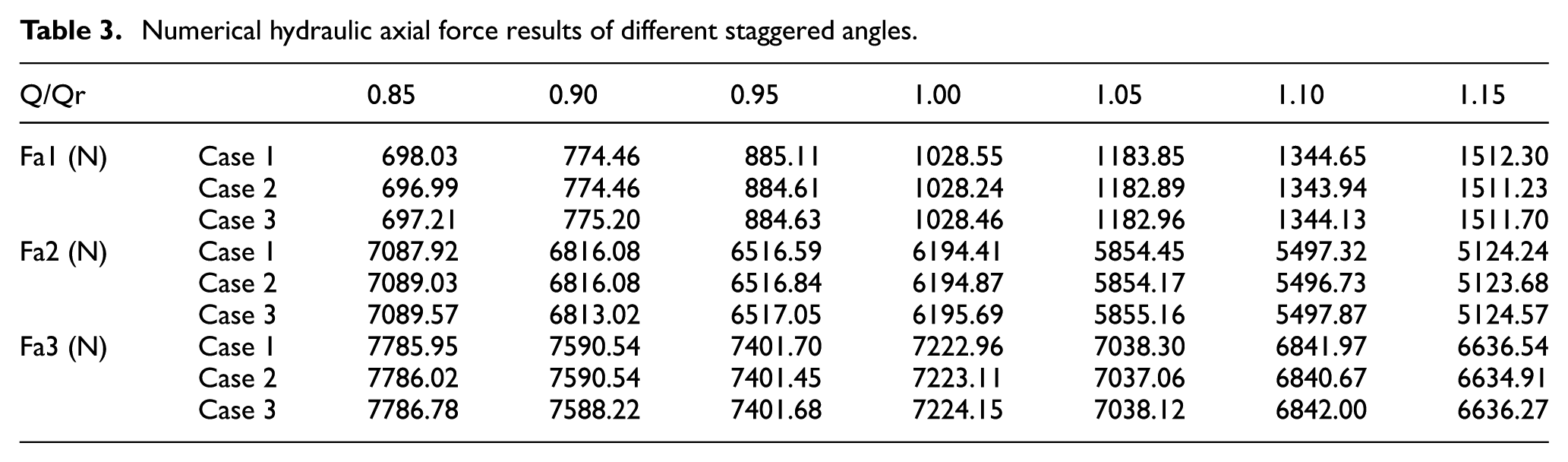
The same situation also appeared for axial force, as shown in Figure 12. The numerical hydraulic axial force results of different staggered angles are shown in Table 3. It can be seen that the staggered angle has almost no influence on pump axial force.

Numerical axial force of different staggered angles: (a) difference between the hub and shroud and (b) momentum axial force and total axial force.
Numerical hydraulic axial force results of different staggered angles.
Different flow rates with the same staggered angle
Three different flow rates with the same staggered angle were discussed. The characteristic curves of a canned nuclear model pump are shown in Figure 13(a)–(c). The maximum efficiency point from largest to smallest is case 4, case 2, and case 5. The corresponding flow rate of the maximum efficiency point from largest to smallest is case 4, case 2, and case 5. The efficiency is approximately the same at 0.9Qr. In 0.85Qr–0.9Qr, the efficiency from largest to smallest is case 5, case 2, and case 4, while in 0.9Qr–1.15Qr, the efficiency is the opposite. The difference is larger near the maximum efficiency point and smaller farther from the maximum efficiency point. The difference between case 5 and case 2 is larger than that between case 4 and case 2. The value and slope are approximately the same in 0.95Qr–1.15Qr for case 2 and case 5. However, the value and slope in case 5 gradually increase in 0.95Qr–0.85Qr. The value of case 4 is larger than the other two in 0.95Qr–1.15Qr, while the slope is the same. The value and slope are gradually reduced in 0.95Qr–0.85Qr and are finally smaller than the other two at 0.85Qr. The power from largest to smallest is case 5, case 4, and case 2. The difference between case 5 and case 4 is smaller than that between case 4 and case 2. Specifically, a different flow rate can produce a different efficiency and head, and the difference is larger than that for staggered angles.

Numerical characteristic curves of the different flow rates: (a) efficiency Q–η curve, (b) head Q–H curve, and (c) power Q–P curve.
The differences in axial force with different flow rates are shown in Figure 14. The difference between the two axial forces acting on the impeller hub and the shroud is shown in Figure 14(a). The difference in momentum axial forces is shown in Figure 14(b), and the total axial forces are shown in Figure 14(c). The value and slope are approximately the same in 0.9Qr–1.15Qr for case 2 and case 5. However, the value and slope of case 5 gradually increase from 0.9Qr to 0.85Qr. The value of case 4 is smaller than the other two in 0.9Qr–1.15Qr, while the slope is the same. The value and slope are gradually reduced in 0.9Qr–0.85Qr and are finally greater than the other two at 0.85Qr. The slopes of the three flow rates are approximately the same. The values of case 2 and case 5 are approximately the same, while that of case 4 is larger than the other two. The value and slope are approximately the same in 0.95Qr–1.15Qr for case 2 and case 5. The value and slope of case 5 gradually increase in 0.95Qr–0.85Qr. The value of case 4 is larger than that of the other two. The slope is the same as the other two in 0.95Qr–1.15Qr, but the value and slope gradually increase from 0.95Qr to 0.85Qr. Specifically, different flow rates can produce different axial forces, and the difference is larger than that of staggered angles.

Numerical axial force of the different flow rates: (a) difference between the impeller hub and shroud, (b) momentum axial force, and (c) total axial force.
Impeller outlet pressure distribution
Three comparisons of pressure distributions at the impeller outlet are shown in Figure 15. It can be seen from Figure 15(a) that the pressure of staggered blade case 2 is different from that of the original blade along the circumferential direction; the difference is not large, but there is a very large difference along the span direction because of the stagger. The difference in staggered angles is shown in Figure 15(b). There is little difference along the circumferential direction for the three staggered angles. The difference mainly appeared along the span direction because of the different angles. The difference in the three flow rates is shown in Figure 15(c). It can be seen that the difference is large for the three blades both in the circumferential direction and in the span direction. This difference explains the differences in hydraulic performance, axial force, and pressure pulsation; these are discussed later.

Pressure distribution at impeller outlet: (a) pressure distribution of the staggered and original blades, (b) pressure distribution of the different staggered angles, and (c) pressure distribution of the different flow rates.
Unsteady CFD results and analysis
To discuss the influence of staggered blades on pressure pulsations in a canned nuclear coolant pump, nine monitoring points were set in the calculation domain, as shown in Figure 16. P10 and P11 were located at the inlet of the impeller. P20 and P21 were located at the outlet of the impeller. P3 is located between the impeller and the diffuser. P4 is located at the outlet of the diffuser. P6 is located in the hub chamber, and P7 is located in the shroud chamber. P5 is located in the annular case, maintaining the same radial direction with P7. The shroud chamber and annular case are connected by a gap. Pressure pulsation coefficient is defined as

Monitoring point distribution.
The model pump frequency domain of the original blade is somewhat similar to other analyses for a pump with a diffuser.23–25 The frequency domain of the staggered blade is somewhat similar to some double-suction pumps. 26 The frequency domain analysis and comparison showed the characteristics of pressure pulsation.
The effects of time step Δt on the simulations are tested. Figure 17 shows the time evolution of the pressure fluctuation on monitoring points P3 and P20 for the two time steps: Δt = 1.6835 × 10⁻⁴ s and Δt = 2.2447 × 10⁻⁴ s. Minimal differences are found among the two time steps. Therefore, by considering the balance between the spectrum accuracy and the computation cost, we denote the final time step as Δt = 2.2447 × 10⁻⁴ s.
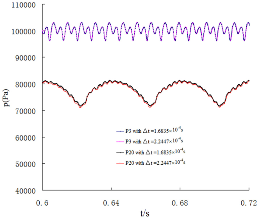
Time evolution of pressure fluctuation on P3 and P20 for two time steps.
Comparison of the staggered and original blades
The pressure pulsation frequency domain of the monitoring points in the impeller for staggered blade case 2 and the original blade is shown in Figure 18. The pressure pulsation maximum amplitude of both blades appeared on 1 × fr at P10, P11, P20, and P21. The maximum amplitude is the same for both blades at the inlet and outlet. At the impeller pass frequency 5 × fr, the amplitude of staggered blade case 2 is smaller than that of the original blade at P10 and P11. The amplitude difference at other frequencies is minimal at the inlet, as shown in Figure 17(a). At diffuser pass frequency 13 × fr, the amplitude of staggered blade case 2 is larger than that of the original blade at P20, while the amplitude of staggered blade case 2 is smaller than that of the original blade at P21. The amplitude difference at other frequencies is minimal at the outlet, that is, staggered blade case 2 produces a different amplitude at impeller pass frequency 5 × fr at the impeller inlet and at diffuser pass frequency 13 × fr at the impeller outlet. Staggered blade case 2 can reduce the amplitude at impeller pass frequency 5 × fr at the impeller inlet.

Monitoring points in impeller: (a) P10 (left) and P11 (right) and (b) P20 (left) and P21 (right).
The pressure pulsation frequency domain of monitoring points in the diffuser and case for staggered blade case 2 and the original blade is shown in Figure 19, respectively. It can be seen in Figure 19(a) that the pressure pulsation maximum amplitude appears at 5 × fr for the original blade and at 10 × fr for the staggered blade case 2 at P3 and P4 in the diffuser. The amplitude appears to be an integer multiple of the impeller pass frequency 5 × fr. At 5 × fr, the amplitude of staggered blade case 2 is obviously smaller than that of the original blade. The amplitudes at other frequencies are approximately the same. There are numerous frequencies at P5 in both cases, as shown in Figure 19(b), but the main frequencies are integer multiples of the impeller pass frequency 5 × fr. The pressure pulsation maximum amplitude appears at 15 × fr for both blades, which is different from P3 and P4. At 5 × fr, the amplitude of staggered blade case 2 is obviously smaller than that of the original blade. However, at 15 × fr, the amplitude of staggered blade case 2 is larger than that of the original blade. The amplitudes at 10 × fr, 20 × fr, 25 × fr, and 30 × fr are not different; that is, staggered blade case 2 produces a different amplitude on impeller pass frequency 5 × fr in the diffuser and reduces the amplitude. At the same time, when changing the position of the maximum amplitude, staggered blade case 2 produces different amplitudes at 5 × fr and 15 × fr in the case and reduces the amplitude at 5 × fr but enlarges the amplitude at 15 × fr.

Monitoring points in the diffuser and case: (a) P3 (left) and P4 (right) and (b) P5.
The pressure pulsation frequency domain of the monitoring points in the hub and the shroud chambers for staggered blade case 2 and the original blade is shown in Figure 20. The pressure pulsation maximum amplitude appears at 5 × fr at P6 and P7 for both blades. The amplitude appears on integer multiples of the impeller pass frequency 5 × fr. At 5 × fr, the amplitude of staggered blade case 2 is smaller than that of the original blade. The amplitudes at other frequencies are approximately the same. Thus, staggered blade case 2 produces different amplitudes at impeller pass frequency 5 × fr in the hub and shroud chambers and reduces the amplitude at the impeller pass frequency 5 × fr.

Monitoring P7 (left) and P8 (right) in the chamber.
Comparison of different staggered angles with the same flow rate
The pressure pulsation frequency domain of monitoring points in the impeller for three staggered blades with different angles is shown in Figure 21. The pressure pulsation maximum amplitude of the three blades appeared at 1 × fr at P10, P11, P20, and P21. The maximum amplitude is the same for three blades at the inlet and outlet. At impeller pass frequency 5 × fr, the amplitude of staggered blade case 2 is at a minimum, the amplitude of case 1 is at a maximum, and the amplitude of case 3 is in the middle at P10 and P11. The amplitude of staggered blade case 3 at 10 × fr and 13 × fr is smaller than that of the other two. The amplitude difference at the other frequencies is small at the inlet, as shown in Figure 21(a). At diffuser pass frequency 13 × fr, the amplitude of staggered blade case 3 is at a minimum, the amplitude of case 1 is at a maximum, and the amplitude of case 2 is in the middle at P20. However, at P21, the amplitude of staggered blade case 2 is at a minimum, the amplitude of case 3 is at a maximum, and the amplitude of case 1 is in the middle. The amplitude difference at other frequencies is also small at the outlet; that is, staggered blades with different angles produce different amplitudes at impeller pass frequency 5 × fr at the impeller inlet and at diffuser pass frequency 13 × fr at the impeller outlet, but the difference is small. Staggered angle 36 can reduce the amplitude at impeller pass frequency 5 × fr at the impeller inlet.
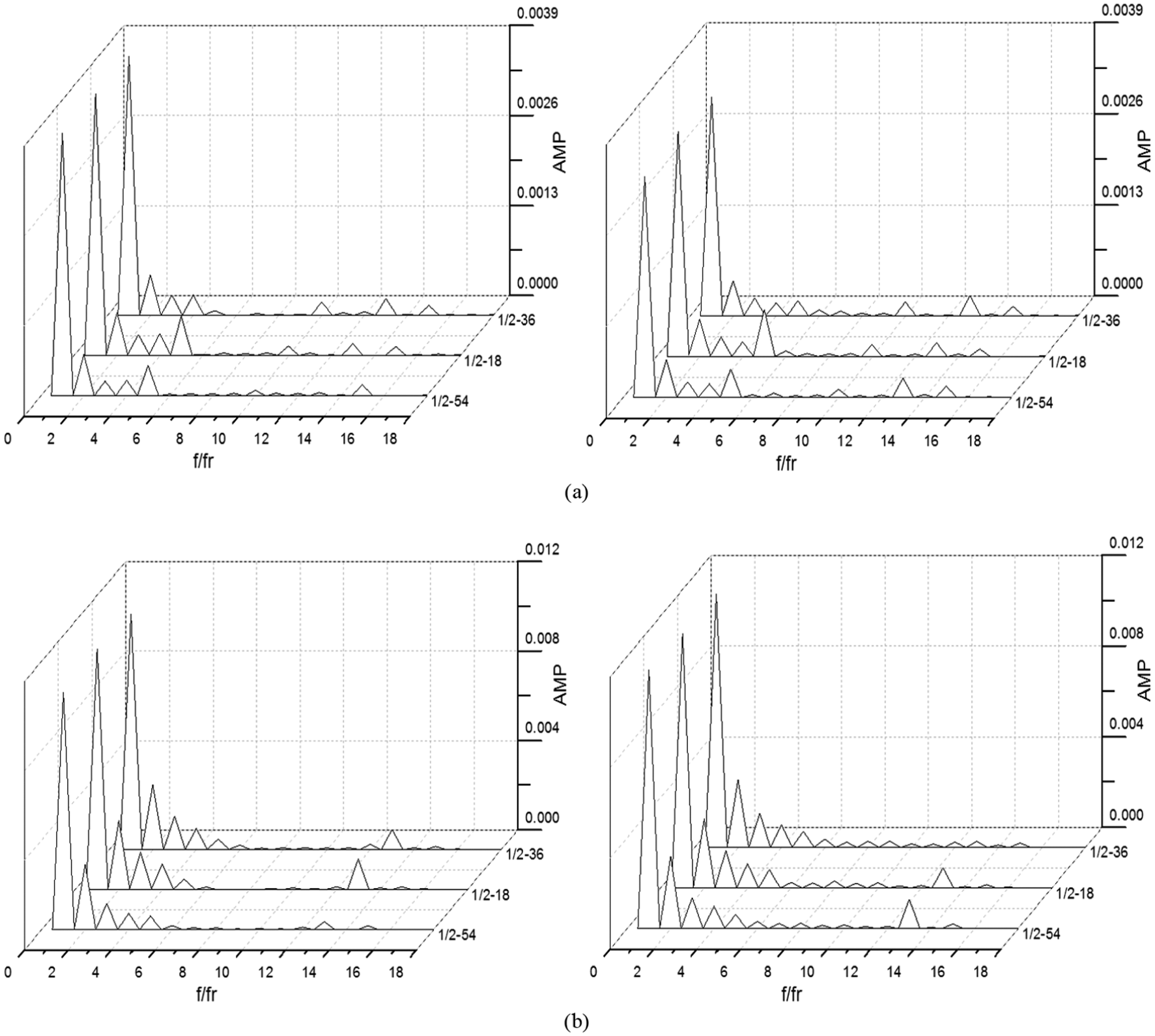
Monitoring points in impeller: (a) P10 (left) and P11 (right) and (b) P20 (left) and P21 (right).
The pressure pulsation frequency domain of the monitoring points in the diffuser and the case of three staggered blades with different angles is shown in Figure 22. It can be seen in Figure 22(a) that the pressure pulsation maximum amplitude appears at 5 × fr for case 1 and case 3 and at 10 × fr for case 2 at P3 and P4 in the diffuser. The amplitude appears as an integer multiple of impeller pass frequency 5 × fr. At 5 × fr, the amplitude of staggered blade case 2 is at a minimum, the amplitude of case 3 is at a maximum, and the amplitude of case 1 is in the middle at P3. The amplitude of staggered blade case 2 is obviously larger than that of the other two at P3 at 10 × fr. The amplitudes at the other frequencies are approximately the same. The amplitude of staggered blade case 2 is obviously less than the other two at P4 at 5 × fr. However, the amplitude of staggered blade case 2 is larger than that of the other two at P4 at 10 × fr. The amplitudes at other frequencies are also approximately the same. There are numerous frequencies at P5 in the case, as shown in Figure 22(b), but the main frequencies are integer multiples of the impeller pass frequency 5 × fr. The pressure pulsation maximum amplitude appears at 15 × fr for the three blades, which was different from P3 and P4. At 5 × fr, the amplitude of staggered blade case 2 is obviously smaller than the other two. However, at 15 × fr, the amplitude of staggered blade case 1 is smaller than that of cases 2 and 3. The amplitudes at 10 × fr, 20 × fr, 25 × fr, and 30 × fr have minimal differences; that is, different staggered angles produce different amplitudes at 5 × fr and 10 × fr in the diffuser, and staggered angle 36 can reduce the amplitude at 5 × fr but enlarges the amplitude at 10 × fr and also changes the position of the maximum amplitude. The staggered angle produces different amplitudes at 5 × fr and 15 × fr in the case and also reduces the amplitude at 5 × fr at staggered angle 36.

Monitoring points in the diffuser and case: (a) P3 (left) and P4 (right) and (b) P5.
The pressure pulsation frequency domain of monitoring points in the hub and shroud chambers for different staggered angles is shown in Figure 23. The pressure pulsation maximum amplitude appears at 5 × fr at P6 and P7 for the three blades. The amplitude appears at integer multiples of impeller pass frequency 5 × fr. At 5 × fr, the amplitude of staggered blade case 3 is at a minimum, the amplitude of case 1 is at a maximum, and the amplitude of case 2 is in the middle at P6. At 10 × fr and 30 × fr, the amplitude of staggered blade case 2 is significantly larger than the other two. The amplitudes at other frequencies have minimal differences. The amplitudes gradually decline for case 2, which is different from the other two at P6. At 5 × fr, the amplitude of staggered blade case 1 is at a minimum, the amplitude of case 3 is at a maximum, and the amplitude of case 2 is in the middle at P7. The amplitudes at other frequencies are approximately the same. Thus, different staggered angles produce different amplitudes at 5 × fr in the hub and shroud chambers. Specifically, different staggered angles produce different amplitudes at 10 × fr and 30 × fr in the hub chamber.

Monitoring P6 (left) and P7 (right) in the chamber.
Comparison of different flow rates with the same staggered angle
The pressure pulsation frequency domain of the monitoring points in the impeller for three staggered blades with different angles is shown in Figure 24. The pressure pulsation maximum amplitude of the three blades appeared at 1 × fr at P10, P11, P20, and P21. At 1 × fr, the maximum amplitude of staggered blade case 4 is smaller than the other two at P10. The amplitude of staggered blade case 5 is at a minimum, the amplitude of case 4 is at a maximum, and the amplitude of case 2 is in the middle at P6 at 1 × fr. At 15 × fr, the amplitude of staggered blade case 4 is significantly smaller than the other two at P10 and P11. The amplitude presents differences at other frequencies at P10 and P11, but the difference is relatively small. At 1 × fr, the maximum amplitude of staggered blade case 4 is smaller than the other two at P20 and P21. At 15 × fr, the amplitude of staggered blade case 4 is significantly larger than the other two. The amplitude presents differences at other frequencies at P10, P20, and P21, but the difference is relatively small, that is, a staggered blade with a different flow produces a different amplitude. The difference is mainly at 1 × fr and 15 × fr in the impeller and is different from the angle.

Monitoring points in impeller: (a) P10 (left) and P11 (right) and (b) P20 (left) and P21 (right).
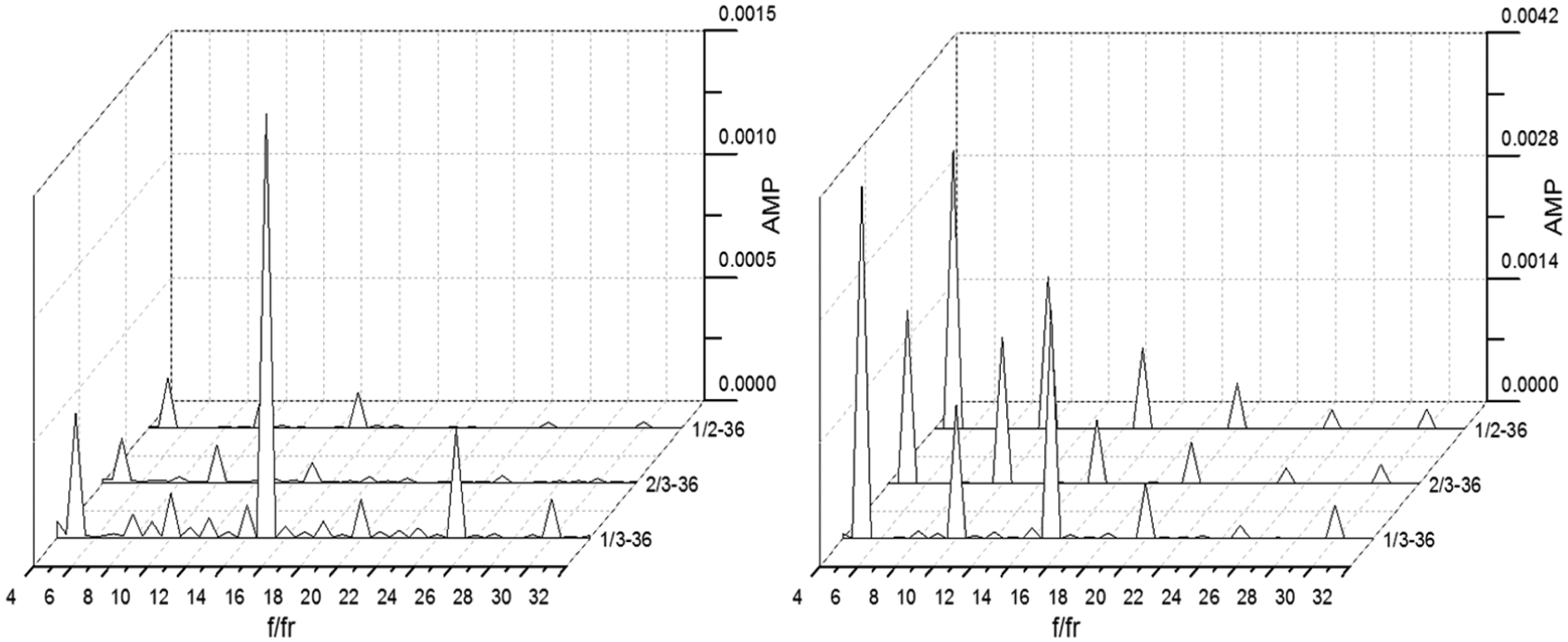
The pressure pulsation frequency domain of the monitoring points in the diffuser and case for three staggered blades with different angles is shown in Figure 25, respectively. The pressure pulsation maximum amplitude appears at 5 × fr at P3 and P4 in the diffuser for case 4 and case 5 and at 10 × fr for case 2. The amplitude appears at integer multiples of impeller pass frequency 5 × fr. At 5 × fr, the amplitude of staggered blade case 2 is at a minimum, the amplitude of case 5 is at a maximum, and the amplitude of case 4 is in the middle at P3. At 15 × fr, the amplitude of staggered blade case 5 is at a minimum, the amplitude of case 4 is at a maximum, and the amplitude of case 4 is in the middle. The amplitude presents a difference at other frequencies at P3, but the difference is relatively small. At 5 × fr, the amplitude of staggered blade case 2 is at a minimum, the amplitude of case 4 is at a maximum, and the amplitude of case 5 is in the middle at P4. At 10 × fr, the amplitude of staggered blade case 5 is at a minimum, the amplitude of case 4 is at a maximum, and the amplitude of case 2 is in the middle. The obvious difference is that the amplitude of staggered blade case 4 is larger than the other two at 15 × fr and 25 × fr at P4. The amplitude presents a difference at other frequencies at P4, but the difference is relatively small. There are numerous frequencies at P5 in the case, but the main frequencies are integer multiples of the impeller pass frequency. The amplitude of staggered blade case 4 is significantly larger than the other two at 5 × fr, 15 × fr, and 25 × fr. Specifically, different flow rates produce different frequencies at integer multiples of the impeller pass frequency 5 × fr in the diffuser and case. Case 2 can reduce the amplitude at 5 × fr; case 4 can increase the amplitude.

Monitoring points in the diffuser and case: (a) P3 (left) and P4 (right) and (b) P5.
The pressure pulsation frequency domain of the monitoring points in the hub and the shroud chambers for different staggered angles is shown in Figure 26. There are numerous frequencies at P6 in the case, but the main frequencies are integer multiples of the impeller pass frequency similar to P5. The amplitude of staggered blade case 4 is significantly larger than the other two at 5 × fr, 15 × fr, and 25 × fr. The pressure pulsation maximum amplitude appears at 5 × fr at P7 for the three blades. The amplitude appears on integer multiples of the impeller pass frequency 5 × fr. At 5 × fr, the amplitude of staggered blade case 5 is at a minimum, the amplitude of case 4 is at a maximum, and the amplitude of case 2 is in the middle. At 10 × fr, the amplitude of staggered blade case 4 is significantly larger than the other two. The amplitudes at other frequencies have minimal differences. The amplitudes gradually decline for cases 2 and 5, which is different from case 4, at P7. Thus, different flow rates produce different amplitudes at 5 × fr and 15 × fr in the hub and shroud chambers. Specifically, case 4 increases the amplitude.
Monitoring P6 (left) and P7 (right) in the chamber.
Analysis of the amplitude difference
We know that the flow at the impeller outlet is nonuniform. The flow at the stator vane acts back on the velocity field in the impeller, which is called “rotor–stator interaction.” These give rise to pressure pulsations, and the frequency and the amplitude are affected by the number of blades and vanes. 3 The staggered blade changes the flow at the impeller outlet and the number of the blades. It makes the pressure distribution staggered both in the circumferential and the parallel directions and doubles the number of blades. Thus, the amplitude of staggered blades is significantly decreased on the impeller and diffuser pass frequencies. The different staggered angles and divided flow make the pressure distribution change in both the circumferential and the parallel directions but do not change the number of blades. Thus, we see that different amplitudes are produced. The angle in case 2 in the middle produces smaller amplitudes at low multiple fr, indicating that the flow at the impeller outlet is more uniform than the other two, but the difference is minimal. The different divided flows make the pressure distribution more nonuniform than the angles. Thus, we see that the amplitude differences are larger. The flow in case 4 makes the pressure distribution more nonuniform than the other two so that the amplitudes are larger. The flow at the impeller outlet can be seen in Figure 15.
Conclusion
In this article, the influence of staggered blades on the hydraulic performance of a canned nuclear pump model is studied using numerical simulations. The agreement between the test and numerical results illustrates that CFD numerical simulations can be used to predict the performance of a canned nuclear pump model with acceptable accuracy. Hydraulic performance curves, axial force curves, and impeller outlet static pressure distributions were obtained. Detailed static pressure pulsations were obtained by setting monitoring points in the flow domain. The performance analysis shows the effect of staggered blades on the pump. The conclusions of this article are as follows:
Staggered blades do not improve hydraulic performance but improve axial force and pressure pulsation. They reduce efficiency, head, and axial force and increase the power slightly relative to the original blade. They reduce the amplitude at impeller pass frequency 5 × fr at the impeller inlet and change the amplitude at diffuser pass frequency 13 × fr at the impeller outlet. They significantly reduce the amplitude at impeller pass frequency 5 × fr in the diffuser and also change the position of the maximum amplitude. They reduce the amplitude at 5 × fr but increase the amplitude at 15 × fr. They reduce the amplitude at impeller pass frequency 5 × fr in the hub and shroud chambers.
The staggered angle has almost no influence on pump hydraulic performance or hydraulic axial force. A staggered blade with different angles can produce different amplitudes. Staggered angle case 2 reduces the amplitude at impeller pass frequency 5 × fr at the impeller inlet and at diffuser pass frequency 13 × fr at the impeller outlet, but the change in the impeller is minimal. It can reduce the amplitude at 5 × fr but increases the amplitude at 10 × fr and changes the position of the maximum amplitude. It can reduce the amplitude at 5 × fr in the case but increases it in the hub chamber.
Different divided flow rates can produce different hydraulic performance and axial forces. For rated flow, the maximum efficiency and head appears in case 4, and the maximum power appears in case 5; the minimal efficiency and power appeared in cases 5 and 2, respectively. For rated flow, case 4 produces the maximal total axial force; the difference in axial forces in the other two blades is minimal. The different divided flows produce different amplitudes. The amplitude change in the impeller is different from the angle above. Case 4 has an increased amplitude in the impeller, diffuser, case, hub chamber, and shroud chamber. Case 2 reduces the amplitude at 5 × fr in the diffuser, and case 5 reduces the amplitude in the shroud chamber at 5 × fr.
The staggered blade changes the flow at the impeller outlet and the number of blades. It makes the pressure distribution staggered in both the circumferential and the parallel direction and doubles the number of blades. The different staggered angles and divided flow make the pressure distribution change both in the circumferential and parallel directions but do not change the number of blades.
Thus, the staggered blade has an important influence on the performance of a canned nuclear coolant pump. Staggered blades do not improve hydraulic performance but improve axial force and pressure pulsation. Specifically, the staggered blade can significantly reduce pressure pulsation amplitude.
Footnotes
Appendix 1
Acknowledgements
Development of the hydraulic components to canned nuclear coolant pump of CAP1400 in the Liaoning Province Science and Technology Innovation Major Project. Principle of shape and performance coordination to canned nuclear coolant pump-independent manufacturing in the National Basic Research Program of China (973 Program).
Academic Editor: Pietro Scandura
Declaration of conflicting interests
The author(s) declared no potential conflicts of interest with respect to the research, authorship, and/or publication of this article.
Funding
The author(s) disclosed receipt of the following financial support for the research, authorship, and/or publication of this article: This research was funded by The Innovation Center of Major Machine Manufacturing in Liaoning.