Numerical simulation of turbulent flow between shrouded contra-rotating disks

Abstract

The turbulent flow between shrouded contra-rotating disks was numerically studied with a two-layer turbulence model and a modified Launder–Sharma low-Reynolds number k-ε model. The dissipation rate decrease caused by solid body rotation was considered in the second model. The comparisons of the effectiveness between these two turbulence models for capturing the critical radius of flow structure transition and reproducing the flow velocity measurements data were presented. For the flow between shrouded disks rotating at the same speed but in opposite senses, that is, the angular velocity ratio of the two disks equals to −1, the Stewartson-type flow structure is found in the cavity. For the flow with one disk rotating more slowly than the other, Stewartson-type flow coexists with Batchelor-type flow, that is, Batchelor-type flow occurs radially outward of the stagnation point where two opposing boundary layer flows meet, and Stewartson-type flow occurs radially inward. The stagnation points near the slower disk move radially outward as the angular velocity ratio decreases toward −1. Theory of rotating fluids with the presence of centrifugal and Coriolis forces stemming from the disk rotation is employed to manifest the flow structure transition mechanisms as the rotation ratio of the disks is varied. The source of the earlier transition to turbulent flow in counter-rotating disk cavity compared with rotor-stator disk cavity is also explained through the research of instability of the flowing free shear layer formed by the counter secondary circulations. With the aid of the numerical results obtained from the two turbulence models, it is found that a more turbulent flow in the core can destroy the Batchelor-type flow and creates a larger Stewartson-type flow region.

Introduction

In most gas turbines, a turbine disk rotates close to either a stationary casing or another co-rotating turbine disk. In some engines, and in some designs of future engines, two adjacent disks may rotate in opposite directions. Such contra-rotating turbines could be used to drive the contra-rotating fans of future generations of ultra-high-bypass-ratio engines. This has the advantage of requiring one fewer row of stator nozzles, thereby reducing the weight and size of the engine. And an additional advantage is that contra-rotating turbine structure can reduce the gyroscopic moment produced during maneuvering flight.^1–3 A superposed radial flow of air is used to cool the turbine disks and to seal the disk cavity. It is important to have a complete understanding of the complicated flow natures and the underlying physics inside contra-rotating disk cavity not only from the point of view of fundamental fluid mechanics but also for the optimization of turbomachinery air-cooling devices.^4,5

The experimental investigations in the rotating cavities are very difficult and expensive. In this situation, numerical simulation becomes an effective method to indirectly understand and predict the behavior of the flow and the heat transfer in the contra-rotating cavity. Numerical modeling of the flow in the rotating cavity turned out to be a difficult problem mostly due to the fact that in the cavity simultaneously exist areas of laminar, transitional, and turbulent flow which are completely different in terms of flow properties. The turbulence model is very important to the simulation of flow and heat transfer inside rotating disk cavity, and the treatment of near-wall turbulent characteristics has obvious effects on the simulation accuracy of flow field in the boundary layer and flow structure in the core region. ⁶ Ji et al. ⁷ and Zhang and Ji ⁸ compared the effectiveness of single-equation turbulence model and Launder–Sharma two-equation turbulence model employed in the near-wall region inside a rotor-stator disk cavity and a co-rotating disk cavity with radial outflow. Craft et al. ⁹ developed a three-dimensional (3D) unsteady version of a low-Reynolds number k-ε model and applied it to a turbulent rotor-stator flow in an enclosed cavity, but this turbulence model required a very fine mesh across the sublayers and also prohibitive time integration preventing from further calculations. For counter-rotating disk cavity, Hill and Ball ¹⁰ presented a direct numerical simulation of turbulent forced convection inside a cylindrical annular enclosure comprising two counter-rotating disks and sidewalls using a Fourier–Chebyshev collocation spectral method. Poncet et al. ¹¹ predicted the turbulent Von Karman flow generated by two counter-rotating smooth flat (viscous stirring) or bladed (inertial stirring) disks using a Reynolds Stress Model (RSM model) and presented comparisons between numerical predictions and Laser Doppler Velocimetry (LDV) measurements. Gan et al. ¹² described a combined experimental and computational study of the zero superposed and superposed flow between contra-rotating disks. The turbulence model used in their computation was based on the low-Reynolds number k-ε turbulence model proposed by Morse^13,14 and exhibited premature transition to turbulent flow. In this article, the two-layer (TL) turbulence model and a modified low-Reynolds number k-ε turbulence model of Launder–Sharma ¹⁵ are employed to numerically study the turbulent flow inside the shrouded contra-rotating disk cavity, and the comparisons of the effectiveness between these two turbulence models for capturing the flow nature inside a contra-rotating disk cavity are presented. Meanwhile, some flow transition characteristics and mechanisms are disclosed.

Physical and mathematical models

Physical model

The schematic of coordinate and physical system adopted in the present simulation is shown in Figure 1, and the computational geometry matches with that of the experimental study carried out by Kilic et al. ¹⁶ and Gan and MacGregor. ¹⁷ The rotating disk cavity system is formed by two disks (disk 1 and disk 2 separated by a spacing of s), with cylindrical shrouds attached to each disk at the outer disk radii. A small axial clearance, s_c, separates the shrouds at the axial midplane allowing each disk/shroud set to rotate freely from the other. Disk 1 rotates clockwise at speed Ω₁, and disk 2 rotates counterclockwise at speed Ω₂. The rotation ratio of disk 2 to disk 1 is denoted by Γ(Γ = Ω₂/Ω₁), which is varied in a range of −1 ≤ Γ ≤ 0. In order to present the rotational effects on the turbulent flow between the shrouded contra-rotating disks, the rotational Reynolds number is defined as Re_ϕ = Ω₁b²/v, where v is the kinematic viscosity of cooling air.

Figure 1.

Schematic of coordinate and physical system.

Governing equations and turbulence models

General formulation

The flow in the shrouded contra-rotating disk cavity is assumed to be steady rotating axisymmetric flow, and it is also assumed that the cooling air is an incompressible fluid with constant properties. The experimental results in the work of Gan and MacGregor ¹⁷ show that the flow in the core is turbulent for Re_ϕ as low as 2.16 × 10⁴. For the parameter range of 6 × 10⁴ < Re_ϕ < 4 × 10⁶ used in the calculation, the flow in the core region inside contra-rotating disk cavity is turbulent. The Reynolds stresses are related to the mean strain rate via an isotropic scalar turbulent viscosity, v_t

$$\overline{V{\prime }_{z}V{\prime }_r}=-v_t(\frac{\partial V_z}{\partial r}+\frac{\partial V_r}{\partial z})$$

(1)

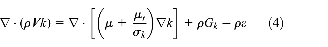
The steady-state Reynolds averaged mass and momentum equations with respect to a reference frame at a rotating velocity Ω can be depicted as

$$\nabla ·\mathit{V}=0$$

(2)

$$\rho (\mathit{V}\nabla )\mathit{V}=-\nabla P+(\mu +{\mu }_t){\nabla }^2\mathit{V}-\rho \Omega \times (\Omega \times \mathbf{r})-2\rho \Omega \times \mathit{V}$$

(3)

where V is the velocity vector (V_r, V_ϕ, V_z), P is pressure, ρ is density, µ is the dynamic viscosity, $-\rho \mathbf{\Omega }\times (\mathbf{\Omega }\times \mathit{r})$ is the centrifugal force, and $-2\rho \mathbf{\Omega }\times \mathit{V}$ is the Coriolis force.

Two k-ε turbulence models were employed in the present simulation, which are the TL turbulence model that includes the standard k-ε turbulence model for the flow in the core region, a single-equation model for the flow near walls, and the modified low-Reynolds number k-ε model of Launder–Sharma ¹⁵ that is able to model the transition from the turbulent core to viscous sublayer close to the wall without the use of special near-wall models.

The TL turbulence model

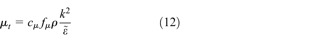
For the core region flow, the standard k-ε turbulence model is used to calculate the turbulent viscosity µ_t as follows

$$\nabla ·(\rho \mathit{V}k)=\nabla ·[(\mu +\frac{{\mu }_t}{{\sigma }_k})\nabla k]+\rho G_k-\rho \epsilon$$

(4)

$$\nabla ·(\rho \mathit{V}\epsilon )=\nabla ·[(\mu +\frac{{\mu }_t}{{\sigma }_{\epsilon }})\nabla \epsilon ]+\frac{\epsilon }{k}[c_{\epsilon 1}{G}_k-\rho c_{\epsilon 2}\epsilon ]$$

(5)

$${\mu }_t=c_{\mu }\rho \frac{k^2}{\epsilon }$$

(6)

where G_k represents the generation of turbulence kinetic energy due to the mean velocity gradients calculated as

$$G_k={\nu }_t[2{\left(\frac{\partial V_z}{\partial z}\right)}^2+2{\left(\frac{\partial V_r}{\partial r}\right)}^2+2{\left(\frac{V_r}{r}\right)}^2+{\left(\frac{\partial V_z}{\partial r}+\frac{\partial V_r}{\partial z}\right)}^2+{\left(\frac{\partial V_{\varphi }}{\partial z}\right)}^2+{\left(\frac{\partial V_{\varphi }}{\partial r}-\frac{V_{\varphi }}{r}\right)}^2]$$

(7)

All the constants c_ε1, c_ε2, c_µ, σ_k, and σ_ε in governing equations have the generally agreed values ¹⁸

$$c_{\epsilon 1}=1.44,c_{\epsilon 2}=1.92,c_{\mu }=0.09,{\sigma }_k=1.0,{\sigma }_{\epsilon }=1.3$$

For the near-wall regions flow, Wolfshtein’s single-equation model ¹⁹ is used to account for the wall proximity effects. In Wolfshtein’s approach, Equation 4 is used to compute k near the wall, and ε and µ_t are obtained as

$$\epsilon =\frac{k^{3/2}}{l_{\epsilon }},{\mu }_t=\rho c_{\mu }\sqrt{k}{l}_{\mu },$$

(8)

by estimating the length scales l_ε and l_µ from

$$l_{\epsilon }=2.55y[1-\exp (-0.263y^{*})]$$

(9)

$$l_{\mu }=2.55y[1-\exp (-0.016y^{*})]$$

(10)

$$y^{*}=\frac{y{k}^{1/2}}{v}$$

(11)

respectively, where y denotes the distance of the closest grid point to the wall. At the wall, k = 0 is set, and at the shroud clearance, $\partial k/\partial z=\partial \epsilon /\partial z=0$ is set.

Modified Low-Reynolds turbulence model of Launder–Sharma

With respect to the performance of the Launder–Sharma turbulence model, there is a tendency for it to predict excessively high levels of near-wall turbulence. ²⁰ The incorporation of the so-called Yap correction for the turbulence length scale and a rotating-related modification for the dissipation rate has led to improved predictions of the velocity distribution for a rotor-stator system, ²¹ but as far as the authors are aware, these modifications have not been applied to contra-rotating disks.

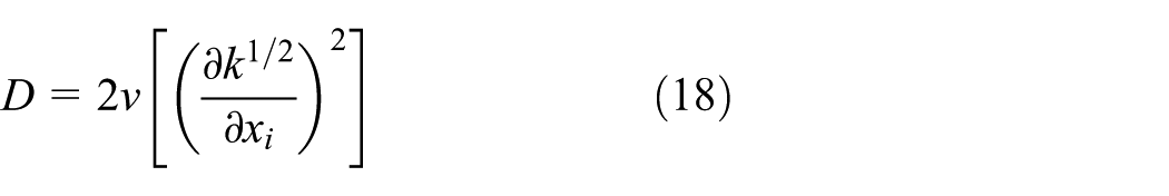
In the Launder–Sharma turbulence model with the incorporation of the Yap correction (LSY), the turbulent viscosity, µ_t, is obtained from

$${\mu }_t=c_{\mu }{f}_{\mu }\rho \frac{k^2}{\tilde{\epsilon }}$$

(12)

$$\nabla ·(\rho \mathit{V}k)=\nabla ·[(\mu +\frac{{\mu }_t}{{\sigma }_k})\nabla k]+\rho G_k-\rho (\tilde{\epsilon }+D)$$

(13)

$$\nabla ·(\rho V\tilde{\epsilon })=\nabla ·\left[\left(\mu +\frac{{\mu }_t}{{\sigma }_{\epsilon }}\right)\nabla \tilde{\epsilon }\right]+\frac{\tilde{\epsilon }}{k}\left[c_{\epsilon 1}{G}_k-\rho c_{\epsilon 2}{f}_2\tilde{\epsilon }\right]+\rho E+Yap$$

(14)

where

$$f_2=1-0.3\exp (-\tilde{R}{e}_t^2)$$

(15)

$$f_{\mu }=\exp [-\frac{3.4}{{(1+0.02\tilde{R}{e}_t)}^2}]$$

(16)

$$\tilde{R}{e}_t=\frac{\rho k^2}{\tilde{\epsilon }\mu }$$

(17)

$$D=2v\left[{\left(\frac{\partial k^{1/2}}{\partial x_i}\right)}^2\right]$$

(18)

$$E=2v{v}_{\mathrm{t}}\left[{\left(\frac{{\partial }^2{u}_j}{\partial x_i\partial x_k}\right)}^2\right]$$

(19)

$$\mathrm{Yap}=\max [0.83\rho \frac{{\tilde{\epsilon }}^2}{k}(\frac{k^{1.5}}{2.55y\tilde{\epsilon }}-1){\left(\frac{k^{1.5}}{2.55y\tilde{\epsilon }}\right)}^2,0]$$

(20)

At the wall, $\partial k/\partial z=\tilde{\epsilon }=0$ is set, and at the shroud clearance, $\partial k/\partial z=\partial \tilde{\epsilon }/\partial z=0$ is set.

Boundary conditions

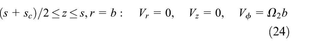
The no-slip boundary conditions on velocity are applied on all the solid walls. The axial and radial velocities are taken to be zero, and the azimuthal velocity is assumed to vary linearly at the shroud clearance

$$z=0,0\le r\le b:V_r=0,V_z=0,V_{\varphi }={\Omega }_{1}r$$

(21)

$$z=s,0\le r\le b:V_r=0,V_z=0,V_{\varphi }={\Omega }_{2}r$$

(22)

$$0\le z\le (s-s_c)/2,r=b:V_r=0,V_z=0,V_{\varphi }={\Omega }_{1}b$$

(23)

$$(s+s_c)/2\le z\le s,r=b:V_r=0,V_z=0,V_{\varphi }={\Omega }_{2}b$$

(24)

$$\left(s-s_c\right)/2\mathrm{<}z\mathrm{<}\left(s+s_c\right)/2,r=b:V_r=0,V_z=0,V_{\varphi }=\frac{1}{2}{\Omega }_{1}b\left(\left(1+\Gamma )+(1-\Gamma \right)\frac{s-2z}{s_c}\right)$$

(25)

Numerical methodology

Numerical computations were based on a finite volume discretization on collocated grids with a staggered arrangement of the variables. The pressure values are stored at the cell centers, while the velocity values are stored at the cell boundaries. For the TL and LSY models, a structured grid of quadrilateral face mesh elements with equidistant nodes was used everywhere, except near the solid surfaces, where the grids were refined. Second-order UPWIND difference scheme was used to discretize momentum, energy, and turbulent transport equations, while the SIMPLE algorithm was introduced for the treatment of the velocity–pressure coupling. The deviation in the maximum value of the effective turbulent viscosity is 0.4% for TL model and 0.3% for LSY model with 30% and 45% more nodes in the radial and axial, respectively. The capabilities and performance of this code have been demonstrated in Chen et al. ²²

Results and discussions

Flow structures at various rotation ratio of the two disks

Figure 2(a) and (b), respectively, presents the contours of stream function Ψ computed with LSY model and TL model for Re_ϕ = 1.25 × 10⁶ and Γ = −0.6. In the Ekman layer attached on each of the two rotating disks, the fluid is pumped radially outward by the combination of the centrifugal force and the radial component of Coriolis force. The outward radial flow along the faster rotating disk 1 is deflected by the shroud, then rolls radially inward along the slower rotating disk 2, pushes against the outward radial flow along disk 2 because of the unbalance radial forces, and then the fluid is forced downward into the core region as well as axially toward the two disks separately. Consequently, a larger clockwise circulation and a weaker counterclockwise circulation separated by the stagnation streamline originating from the stagnation point (at a nondimensional radius x_st = r_st/b near the slower rotating disk) are formed in the r-z plane. Both turbulence models can describe the flow structure except the location of the stagnation point (to be discussed in more detail in the section “The critical radius of flow structure transition for −1 < Γ < 0”).

Figure 2.

Contours of stream function modeled using the (a) LSY and (b) TL models for Re_ϕ = 1.25 × 10⁶ and Γ = −0.6.

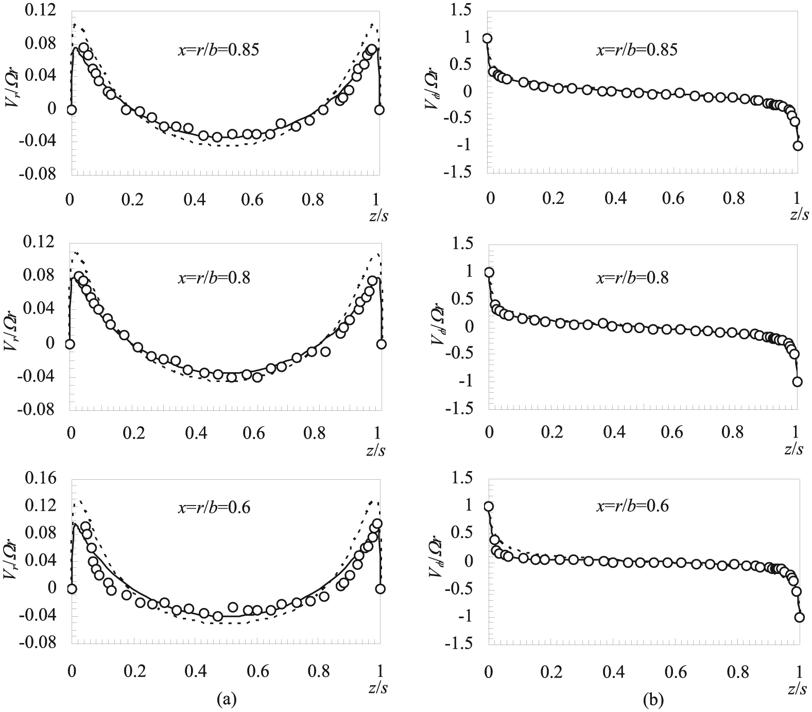
Figure 3 shows the axial profiles of V_r/Ωr and V_ϕ/Ωr corresponding to the conditions in Figure 2. From Figure 3(a) and (b), it can be seen that radial inward flow occurs across the entire interior core, and the tangential velocity varies almost linearly with the axial position (z/s) in the core region at r/b = 0.6. The flow structure is of Stewartson type. ²³ At r/b = 0.85, The region near the axial midplane (0.3 < z/s < 0.7) is characterized by a quasi zero radial velocity and a constant tangential velocity. The angular speed of the rotating core increases slightly with increasing radial distance (V_ϕ/Ωr = 0.2 for r/b = 0.85 and V_ϕ/Ωr = 0.25 for r/b = 0.9). This is consistent with the Batchelor-type flow characteristic. ²⁴ In fact, the Stewartson-type flow holds near the center region, while the Batchelor-type flow is limited to the periphery region of the disk cavity for −1 < Γ < 0. The flow structure transition is associated with the two-cell structure as described above, that is, Stewartson-type flow occurs radially inward of the stagnation point and Batchelor-type flow radially outward. Both turbulence models yield qualitative agreement with Kilic’s experiment predictions ¹⁶ for this transition.

Figure 3.

Axial profiles of V_r/Ωr and V_ϕ/Ωr for Re_ϕ = 1.25 × 10⁶, Γ = −0.6: (a) V_r/Ωr and (b) V_ϕ/Ωr.

Figure 4(a) and (b), respectively, present the contours of stream function Ψ computed with LSY model and TL model for Re_ϕ = 3.93 × 10⁵ and Γ = −1. Owing to the centrifugal force and the radial component of Coriolis force, the air near contra-rotating disk walls flows radially outward to the shrouds and turns inward at the shrouds clearance, then meets to form an inflowing free shear layer in the midplane (z/s = 1/2), and ultimately flows axially to the adjacent disk from the free shear layer. The mean secondary flow in the r-z plane thus consists of two large counter recirculation cells, with the centers of circulating cells occurring near the shrouds (x = r/b = 0.95 for LSY model and x = r/b = 0.935 for TL model).

Figure 4.

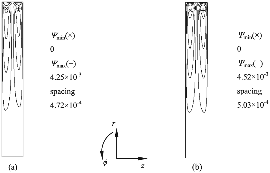
Contours of stream function modeled using the (a) LSY and (b) TL models for Re_ϕ = 3.93 × 10⁵ and Γ = −1.

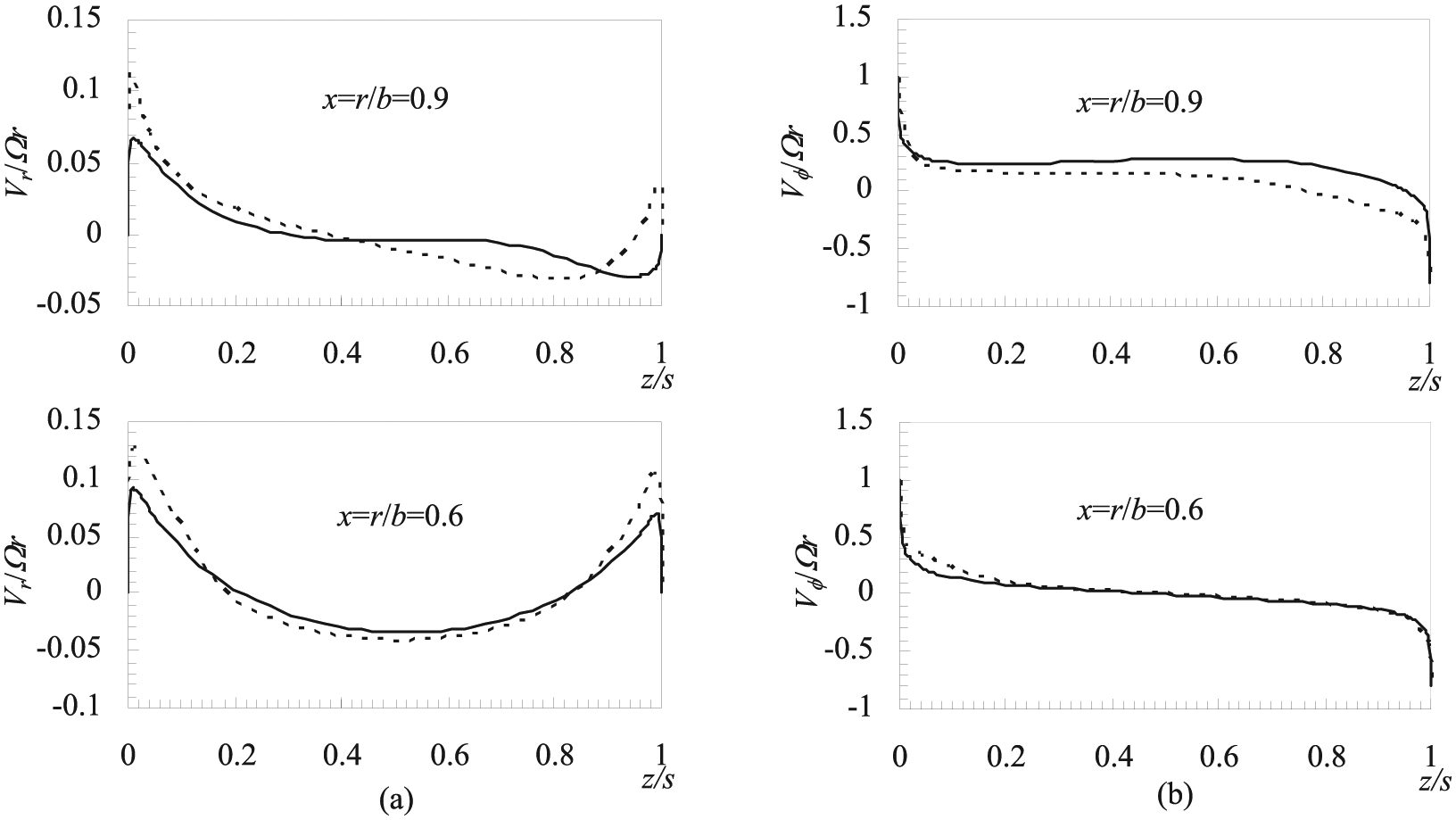
Figure 5 shows the axial profiles of V_r/Ωr and V_ϕ/Ωr corresponding to the conditions in Figure 4. From Figure 5(a), it is seen that there is no radial inward “jet” at the midplane same as Batchelor-type flow. Instead, radial inward flow occurs over the entire region between the two boundary layers. From Figure 5(b), it is seen that the tangential velocity in the core region varies almost linearly with the axial position, z/s, and there is no rotating core between the disk boundary layer and the free shear layer as Batchelor ²⁵ predicted. Obviously, the flow between the contra-rotating disks at the same speeds is of a Stewartson type. ²³ Both the predictions of the two turbulence models agree with the Stewartson-type flow structure as obtained in Gan’s experiment. ¹⁷

Figure 5.

Axial profiles of V_r/Ωr and V_ϕ/Ωr for Re_ϕ = 3.93 × 10⁵, Γ = −1: (a) V_r/Ωr and (b) V_ϕ/Ωr.

The critical radius of flow structure transition for −1 < Γ < 0

As discussed above, Stewartson-type flow occurs radially inward of the stagnation point and Batchelor-type flow radially outward for −1 < Γ < 0. The location of the stagnation point can be obtained by inspecting the sign change of the radial velocity component near the slower rotating disk 2. Figure 6 shows the axial distribution of V_r/Ωr at x = r/b = 0.7 and x = r/b = 0.75 calculated with the LSY model for Re_ϕ = 1.25 × 10⁶ and Γ = −0.6. The V_r/Ωr at x = 0.7 is positive near disk 2, indicating that the flow there is radially outward. The radial velocity profile at x = 0.75 is negative near disk 2, indicating that the flow is radially inward at that location. Thus, the stagnation point occurs between 0.7 < x_st < 0.75 for the LSY turbulence model. Figure 7 shows the axial distribution of V_r/Ωr at x = r/b = 0.8 and x = r/b = 0.85 calculated with TL model corresponding to the conditions in Figure 6. The V_r/Ωr at x = 0.8 is positive near disk 2, and the radial velocity profile at x = 0.85 is negative near disk 2. Thus, the stagnation point occurs between 0.8 < x_st < 0.85 for the TL turbulence model. Calculations for the locations of the stagnation points were made at other values of Γ in addition to those shown here for Re_ϕ = 1.25 × 10⁶, and the results are shown in Table 1, accompanied by the experimental data from Kilic et al. ¹⁶ Both the computations and measurements predict the fact that the nondimensional critical radius of flow structure transition x_st increases as the rotation ratio Γ decreases. However, the numerical results from LSY turbulence model match the experimental data much better than that for TL turbulence model, although the location of the stagnation point for Γ = −0.4 could not be confirmed by Kilic because no measurements were made for x < 0.6 in their experiments. Obviously, TL turbulence model predicts larger values of x_st, that is, TL turbulence model predicts larger domains of Stewartson-type flow.

Figure 6.

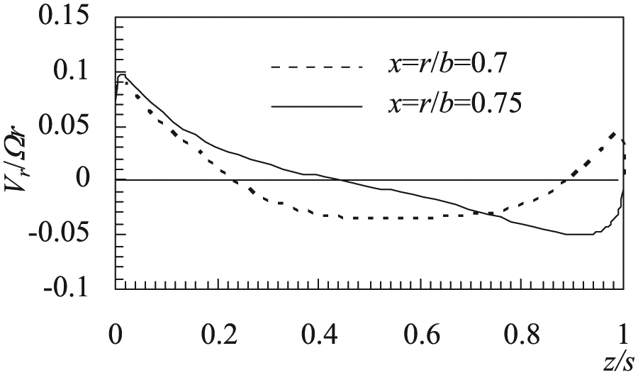
Axial profiles of V_r/Ωr at x = 0.7 and x = 0.75 modeled using the LSY model, Re_ϕ = 1.25 × 10⁶, Γ = −0.6.

Figure 7.

Axial profiles of V_r/Ωr at x = 0.8 and x = 0.85 modeled using the TL model, Re_ϕ = 1.25 × 10⁶, Γ = −0.6.

Table 1.

The locations of the stagnation points.

	Γ = −0.4	Γ = −0.5	Γ = −0.6	Γ = −0.8
Experimental data 16	xst < 0.6	xst = 0.6	xst = 0.75	xst = 0.85
Results of LSY	0.45 < xst < 0.5	0.55 < xst < 0.6	0.7 < xst < 0.75	0.85 < xst < 0.9
Results of TL turbulence model	0.55 < xst < 0.6	0.65 < xst < 0.7	0.8 < xst < 0.85	0.9 < xst < 0.95

LSY: Launder–Sharma turbulence model with the incorporation of the Yap correction; TL: two-layer.

The quantitative prediction of V_r/Ωr and V _$\varphi$ /Ωr

From Figures 3 and 5 it can be seen that at all values of x = r/b considered in this study, there is good agreement between the computed and measured velocities for both the radial and tangential components of velocity for LSY turbulence model. However, for TL turbulence model, the peak value of V_r/Ωr in the boundary layers is higher than that measured, and the tangential velocity in the rotating core is lower than that measured even though it is well predicted in the Stewartson-type flow region. The computed axial distributions of V_r/Ωr and V_ϕ/Ωr for Γ = −0.2, −0.4, and −0.8 shown in Figures 8–10, respectively, support the result. When the flow becomes more turbulent, the peak value of V_r/Ωr is increased as a result of stronger momentum exchange between the boundary layer and the core flow, and V_ϕ/Ωr in the rotating core is decreased as a result of energy dissipation. This indicates that the viscous effects are slightly underestimated by the TL turbulence model because the underestimated viscous effects cause the flow to become fully turbulent earlier than the actual experimental results.

Figure 8.

Computed axial profiles of V_r/Ωr and V_ϕ/Ωr for Re_ϕ = 1.25 × 10⁶, Γ = −0.2: (a) V_r/Ωr and (b) V_ϕ/Ωr.

Figure 9.

Computed axial profiles of V_r/Ωr and V_ϕ/Ωr for Re_ϕ = 1.25 × 10⁶, Γ = −0.4: (a) V_r/Ωr and (b) V_ϕ/Ωr.

Figure 10.

Computed axial profiles of V_r/Ωr and V_ϕ/Ωr for Re_ϕ = 1.25 × 10⁶, Γ = −0.8. (a) V_r/Ωr and (b) V_ϕ/Ωr.

The quantitative prediction of turbulent quantities

The turbulent viscosity fields predicted by the two turbulence models are shown in Figures 11 and 12. The maximum turbulent viscosity is located at the center at about x = r/b = 0.7 for Γ = −0.6 and moves radially outward for Γ = −1. The locations of the minimum turbulent viscosity are at the wall for all conditions. The distributions of the turbulent viscosity predicted by the LSY and TL models are similar; however, the maximum value of the turbulent viscosity predicted by TL model is larger than that predicted by the LSY model by 72% and 60% for Γ = −0.6 and Γ = −1, respectively. The axial distributions of turbulent viscosity µ_t at x = r/b = 0.6 for different conditions are compared in Figure 13 for the two turbulence models. It is also clear that the TL model predicts much larger values of µ_t both in the boundary layer and in the core region than the LSY model. Therefore, it is verified that TL turbulence model predicts a more turbulent flow inside contra-rotating disk cavity compared to the LSY model. In conjunction with the forgoing result that TL model predicts a larger Stewartson-type flow region compared to the LSY model and experimental measurements, it can be concluded that a more turbulent flow in the core has destroyed the Batchelor-type flow and creates a larger Stewartson-type flow region.

Figure 11.

Contours of µ_t computed with the (a) LSY and (b) TL models for Re_ϕ = 1.25 × 10⁶ and Γ = −0.6.

Figure 12.

Contours of µ_t modeled using the (a) LSY and (b) TL models for Re_ϕ = 3.93 × 10⁵ and Γ = −1.

Figure 13.

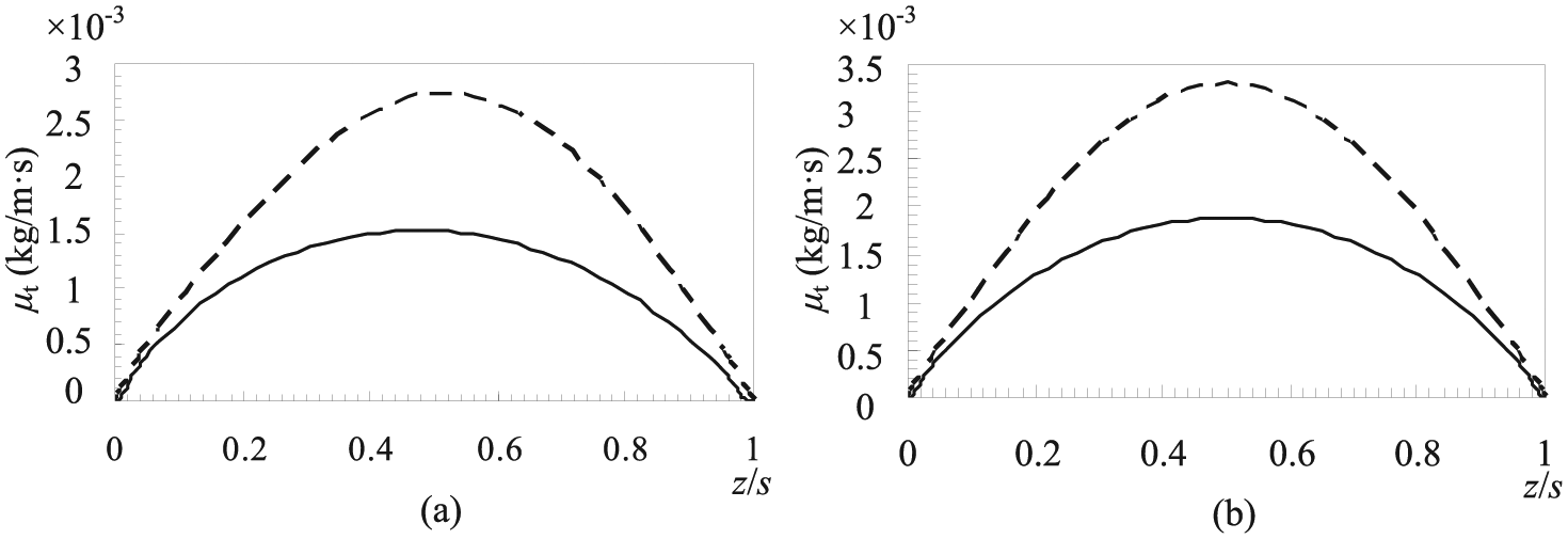
Axial distributions of µ_t at x = r/b = 0.6 for (a) Re_ϕ = 1.25 × 10⁶, Γ = −0.6 and (b) Re_ϕ = 3.93 × 10⁵, Γ = −1.

The mechanisms of flow structure transition

In equation (3), with V  = V_re_r + V_ϕe_ϕ + V_ze_z, Ω = Ωe_z, and e_r, e_ϕ, and e_z denoting unit vectors in radial, tangential, and axial directions, respectively, the centrifugal force and the Coriolis force can be expressed, respectively, as follows

$$-\rho \mathbf{\Omega }\times (\mathbf{\Omega }\times \mathit{r})=\rho {\Omega }^{2}r{e}_r$$

(26)

$$-2\rho \mathbf{\Omega }\times \mathit{V}=2\rho \Omega V_{\varphi }{e}_r-2\rho \Omega V_r{e}_{\varphi }$$

(27)

from which one can see the centrifugal force lies in radially outward direction and the Coriolis force has one radial component 2ρΩV_ϕe_r and one tangential component −2ρΩV_re_ϕ. With the same sign of Ω and V_ϕ, the radial component 2ρΩV_ϕe_r is positive and radially outward.

For the case of Γ = −1, the radial velocities are positive in the Ekman layer on the counter-rotating disks due to the radially outward centrifugal force and Coriolis force, and are negative in the core region between the two boundary layers due to the deflecting effects of the shrouds. So the tangential viscous forces near the two disks are in opposite direction with Ω₁ = −Ω₂. The tangential component of Coriolis force is also of opposite directions both in the boundary layers on the two disks and in the core region with Ω₁ = −Ω₂ and V_r1 = V_r2. As a result, the inward radial flow penetrates the core region and the opposite rotating flows on either hand side of the axial midplane are neutralized, which is the forming mechanism of the Stewartson-type flow for the case of Γ = −1.

As illustrated schematically in Figure 14, the tangential component of Coriolis force on the fluid on left hand side of the axial midplane can be calculated as −2ρΩ₁V_r1, which is positive with positive Ω₁ and negative V_r1, while the tangential Coriolis force on the fluid on right hand side can be calculated as −2ρΩ₂V_r2, which is negative with negative Ω₂ and V_r2. So the tangential Coriolis forces on both sides of the axial midplane are of the same magnitude but in opposite direction. The coupling of the opposite tangential Coriolis forces generates tangential velocity gradient in axial direction and tears fluid circumferentially. As a result, the flows between the counter-rotating disks appear more chaotic and tumbling, which provided the interpretation for Gan and MacGregor’s ¹⁷ experiment result that the flow in counter-rotating disk cavity transits earlier to turbulent compared with rotor-stator disk cavity.

Figure 14.

Sketches of the coupling effects of the opposite tangential Coriolis forces for Γ = −1: (a) left hand of the axial midplane and (b) right hand of the axial midplane.

For the case of −1 < Γ < 0, the fluid near the faster rotating disk 1 moves toward disk 2 as well as radially inward. As a consequence, the radial velocity is quasi-zero in the core region and the fluid is brought on rotation with disk 1 like a sandwich via the combined effects of tangential viscous force near disk 1 and tangential components of the Coriolis force near disk 2 for x ≥ x_st. This is known as the Batchelor flow structure. With the sandwich-like rotating core acting in the same way as the rotating shroud, the forming mechanism of the Stewartson-type flow structure follows the same philosophy as that for Γ = −1 for x ≤ x_st.

Conclusion

The modified Launder–Sharma low-Reynolds number k-ε model could more accurately describe the critical radius of flow structure transition and reproduce the flow velocity measurement data than the TL turbulence model. The TL turbulence model predicts a more turbulent flow and a larger Stewartson-type flow region compared to the former turbulent model and experimental measurements. The Stewartson-type flow occurs radially inward of the stagnation point and the Batchelor-type flow radially outward for −1 < Γ < 0. The stagnation points near the slower disk move radially outward as Γ decreases, and the Stewartson-type flow occupies the entire region for Γ = −1. The flow structure transition originates from the change of the rotating forces in the flow field as the rotation ratio of the disks is varied. The couple of the opposite tangential Coriolis forces tears fluid circumferentially and generates more turbulence in the flow between the disks at counter-rotation. A more turbulent flow in the core can destroy the Batchelor-type flow and creates a larger Stewartson-type flow region.