Modeling and optimization of industrial multistage compressed air system using actual variable effectiveness in hot regions

Abstract

In this article, modeling and optimization of power consumption of two-stage compressed air system have been investigated. To do so, the two-stage compressed air cycle with intercooler of Fajr Petrochemical Company was considered. This cycle includes two centrifugal compressors, a shell, and a tube intercooler. For modeling of power consumption, isentropic efficiencies of actual compressors and thermal effectiveness of intercooler are calculated from experimental data. In these equations, isentropic efficiency of compressors is a function of the inlet temperature, and thermal effectiveness of the intercooler is a function of the inlet air temperature, inlet water temperature of the intercooler, and inlet volumetric flow rate of the cycle. For optimization of power consumption, the Lagrangian method is used. Power consumption and isentropic efficiency of the first- and second-stage compressors, thermal effectiveness of the intercooler, and entropy generation of compressors are considered as the objective function and optimization conditions, respectively. In comparison with the experimental data, the modeling provided suitable accuracy. The optimization effectively reduced the power consumption of the cycle, especially in summer, in a way that the minimum and maximum reductions were 2.9% and 9.6%, respectively.

Introduction

Air compressors are used in variety of industries to supply process requirements, operate pneumatic tools and equipments, and meet instrumentation needs. Compressed air systems use about 10% of the total industrial energy use in the world. Also, these systems are typically one of the most expensive utilities in an industrial facility.^1,2 Some large compressors require several kilowatt powers to run. Even for a small air compressor with a displacement of 10 m³/min, an electrical motor of power 50–100 kW is required.^3–5

The work input to a compressor is minimized when the compression process is executed in an internally reversible manner. When the changes in kinetic and potential energies are negligible, the compressor work is given by $\int \mathrm{vdp}$ . ⁶ Obviously, one way of minimizing the compressor work is to approximate an internally reversible process as much as possible by minimizing the irreversibilities such as friction,^7,8 turbulence,^9,10 and nonquasi-equilibrium compression. The extent to which this can be accomplished is limited by economic considerations. A second (and more practical) way of reducing compressor work is to keep the specific volume of the gas as small as possible during the compression process. This is done by maintaining the temperature of the gas as low as possible at the inlet of compressor and during compression since the specific volume of a gas is proportional to temperature.

There are some regions in the world with specific climatic conditions such as large differences in minimum and maximum temperatures during a year. These temperature variations can cause considerable difference in power consumption and performance of air compressors. These conditions lead to power consumption fluctuations of up to about 15%.^11–14

For large or middle power compressors, one of the most important ways to save energy is using multistage compression and intercooling.^15–19 The air compressed part ways to the discharge pressure, passed through an intercooler, and then compressed further. To minimize specific work input or power consumption, in two-stage air compression with 100% isentropic efficiency and 100% intercooler effectiveness, is readily seen to require that the stage pressure ratio rise should be the square root of overall pressure ratio in the more restrictive perfect gas model.

Lewins ²⁰ modeled and optimized a multistage compressor with an intercooler for an ideal gas model. He used Lagrange method of optimization to find optimum condition. He showed that working in the perfect gas model, in which leads to some basic results in an optimization of a gas turbine that gives maximum work per unit mass circulated. These are useful for giving a feel to more realistic results in gas turbine and Joule cycle theory. It has been recently shown that the essence of these results remains true, albeit with a different emphasis, when the model is relaxed to the ideal gas only. Those results have been given for a Joule cycle optimized for maximum specific work. Also, he showed that if the stage duties vary, optimal condition can be calculated as a function of isentropic efficiencies of compressors and effectiveness of intercoolers.

Consequently, due to the supercritical heat rejection of the trans-critical cycle and the slopes of the isotherms in the supercritical region, the highest efficiency may be achieved at pressure ratios of the first- and second-stage compressors significantly different from each other, depending on the operating conditions. ²¹ In actual condition, the isentropic efficiencies of compressors are not constant and have significant variations with operational condition. ²² Compressor efficiency, pressure ratio, and inlet air temperature are three important parameters in optimization of power consumption in multistage compressors. ²³

Wu et al. ²⁴ optimized a multistage air compression system with a shell and a tube intercooler. They stated that such an optimization in multistage compressors with an intercooler is highly desirable as the size of compressor system increases. Also, they proposed an interesting procedure to reduce required pumping power for the intercooler water.

Ghorbanian and Gholamrezaei ²⁵ used an artificial neural network (ANN) for compressor performance prediction. Their results show that if one considers a tool for interpolation and extrapolation applications, multilayer perception network technique is the most powerful candidate. Furthermore, for the prediction of the compressor efficiency, ANN is a powerful technique.

Al-Doori ²⁶ investigated the effect of important parameters on the performance of gas turbine power plant. He focused on different parameters including different compressor pressure ratios, different ambient temperatures, air–fuel ratio, turbine inlet temperature, and the cycle peak temperature ratio. He showed that an increase in pressure ratio in each compressor would enhance the cycle’s produced work. Also, any increase in ambient temperature increases power consumptions and reduces the cycle work. Therefore, increasing ambient temperature can deteriorate thermal efficiency.

Unfortunately, there is a serious shortage in the literature about air compressed system in hot region and effect of the inlet temperature on isentropic efficiencies of compressor and intercooler effectiveness. Therefore, in this article, power consumptions of two-stage air compressed cycle in hot regions have been modeled and optimized by considering variation in ambient temperature, variation in isentropic efficiencies, and intercooler effectiveness.

Material and methods

Compressed air system specifications

The compressed air cycle that has been investigated in this article is placed in Fajr Petrochemical Company (Mahshahr, Iran) and includes two centrifugal compressors, a shell, and a tube heat exchanger as intercooler. Table 1 shows operating parameters of both compressors in summer condition. The investigated intercooler is a water-cooled shell and tube heat exchanger from Siemens. The outlet air from intercooler would be dried with an industrial dryer to fix air moisture content. Thus, it is assumed that air moisture content would be constant in compression process. Table 2 demonstrates the operating parameters of intercooler.

Table 1.

Operating parameters of compressors (summer condition).

Parameters	First compressor	Second compressor
Inlet air pressure (bar)	1	1.91
Inlet air temperature (K)	321	321
Inlet air flow rate (m3/s)	8.70	4.61
Heat (kJ/kg)	74.7	62.30
Outlet air pressure (bar)	2.03	3.46
Outlet air temperature (K)	409	396
Power consumption (kW)	848	685

Table 2.

Operating parameters of intercooler heat exchanger (design condition).

Parameters	Value
Inlet cooling water pressure (bar)	4.2
Inlet cooling water temperature (K)	296
Outlet cooling water temperature (K)	305
Outlet cooling water flow rate (m3/s)	170

To measure thermodynamic parameters such as pressure, moisture content, and flow rate, a Testo 400 device with three probes for each parameter was used. Measurement accuracy of the device is 0.1°C, 0.001 bar, and 0.1 m³/h for temperature, pressure, and flow rate, respectively. Also, a Fluke 1735 power analyzer device with data logger for compression power measuring in each compressor was implemented. Pressure ratios in compressors are variable with temperature, as overall pressure of the cycle sometimes is 3.8 bar (in winter) and 3.49 bar (in summer).

Thermodynamic modeling

Figure 1 shows the components of a two-stage compressor with a single intercooler. For the thermodynamics modeling of power consumption of compressors, we assumed that the air is ideal gas and includes moisture. Also, compression processes in the first- and second-stage compressors are adiabatic.

Figure 1.

Two-stage intercooled compressing system.

First compressor

We know from experimental results that the isentropic efficiency of compressor is the ratio of enthalpy differences in isentropic condition to enthalpy differences in actual conditions

$${\eta }_{12}=\frac{\Delta h_{ise}}{\Delta h_{act}}=\frac{h_{2s}-h_1}{h_2-h_1}$$

(1)

In thermodynamic modeling of power consumption, the hypothesis of ideal gas model by considering the humidity of air is used. The effects of air humidity have to be considered as well. Humid air can be considered as a mixture of dry air and water vapor. The water vapor is assumed to be near liquefying, and humid air is treated as an ideal gas. Using equations (2) and (4), the enthalpy of humid air based on hypothesis of ideal gas model should be calculated ²¹

$$\frac{T_{2s}}{T_1}={\left(\frac{P_{2s}}{P_1}\right)}^{\frac{k-1}{k}}$$

(2)

$$\varphi =\frac{P_{\mathrm{vap}}}{P{\prime }_{\mathrm{vap}}}$$

(3)

$${P^{\prime }}_{vap}\left(T\right)=P_{cr}\exp \left(\frac{T_{cr}}{T}\left(-7.85\tau +1.84{\tau }^{1.5}+22.67{\tau }^{3.5}-15.93{\tau }^4+1.77{\tau }^{7.5}\right)\right)$$

(4)

With the evaluation of the mole fraction of water vapor in humid air, the specific heat capacity and consequently isentropic power consumption can be calculated

$$X_{\mathrm{va}p}=\frac{P_{\mathrm{vap}}}{P_1}=\frac{\varphi P{\prime }_{\mathrm{vap}}}{P_1}$$

(5)

$$c_{\mathrm{pw}}\left(T\right)=a_w+b_w\left(T\right)+c_w{\left(T\right)}^2+d_w{\left(T\right)}^3$$

(6)

$$c_{\mathrm{pa}}\left(T\right)=a_a+b_a\left(T\right)+c_a{\left(T\right)}^2+d_a{\left(T\right)}^3$$

(7)

$$c_{p,\mathrm{ha}}=X_{\mathrm{vap}}{c}_{\mathrm{pw}}+(1-X_{\mathrm{vap}})c_{\mathrm{pa}}$$

(8)

$$W_{12\mathrm{act}}=\frac{m^{·}(c_{p,\mathrm{ha}}\left(T_{2s}\right)T_{2s}-c_{p,\mathrm{ha}}\left(T_1\right)T_1)}{{\eta }_{12}}$$

(9)

Using the method of least square error, the isentropic efficiency of the compressor as a function of the inlet temperature can be calculated from the experimental data with a two-degree polynomial fit

$${\eta }_{12}\left(T_1\right)=0.000006948T_1^2-0.0050537T_1+1.6123$$

(10)

Intercooler

The aim of modeling of intercooler in a compressed air system is calculating its thermal effectiveness (equation 11) and outlet air temperature

$$\epsilon =\frac{T_2-T_3}{T_2-T_1}$$

(11)

To calculate the effectiveness of intercooler, the outlet air temperature should be determined. Unlike some studies^26,27 that assumed the effectiveness equal to quantity and constant, using equation (11), thermal effectiveness could not be constant.

According to recorded empirical data for this cycle, the best method for calculating the outlet air temperature and computation of thermal effectiveness is ANN method. To use ANN, 256 different recorded data for intercooler were implemented.

Regarding the different networks and using trial-and-error method, the best network for intercooler is a feed-forward network by two hidden layers. Transfer function of the first layer is tangent sigmoid with 20 hidden neurons, and the second layer is log sigmoid with the same number of hidden neurons.

To update weight factor and bios in the first hidden layer, trainlm function in Levenberg–Marquardt optimization method was used, and Leamgdm training function has been implemented for the second layer that is a suitable method to reduce inclined plane to train and update weight and bios. To train the network, we used train function in which the number of trained data is 70% of the total number of data. A total of 15% of data to test and 15% of them for network validation were chosen randomly.

Second compressor

Power consumption of the second compressor depends on the thermal effectiveness of intercooler. Power consumption calculation procedure of this compressor is same as that of the first compressor. Also, since we have a dryer next to intercooler, the inlet air moisture for the second compressor is equal to that of the first compressor. The governing equation of the second compressor is similar to that of the first compressor.

Here, we can use a polynomial as a function of the inlet air temperature to determine the isentropic efficiency of the second compressor, as same as the first compressor. Therefore, using experimental data, isentropic efficiency can be calculated

$${\eta }_{34}\left(T_3\right)=0.00489246T_3^2-3.134729T_3+572.427$$

(12)

Optimization of power consumption

For optimization of the cycle, Lagrange multipliers were used. So, we introduce further Lagrange multipliers and distinguish between the efficiency of the first- and second-stage compression. Writing the objective function as

$$W\equiv L_0=h_2-h_1+h_4-h_3$$

(13)

Together with constraints and their Lagrange multipliers

$$L_a\equiv \lambda [R\ln \left(r\right)-\underset{T_1}{\overset{T_{2s}}{\int }}\frac{\mathrm{dh}}{T}-\underset{T_3}{\overset{T_{4s}}{\int }}\frac{\mathrm{dh}}{T}]$$

(14)

$$L_b\equiv \chi [{\eta }_{12}-\frac{h_{2s}-h_1}{h_2-h_1}]$$

(15)

$$L_c\equiv \mu [\epsilon -\frac{h_2-h_3}{h_2-h_1}]=\mu [\epsilon -1+\frac{h_3-h_1}{h_2-h_1}]$$

(16)

$$L_d\equiv \kappa [{\eta }_{34}-\frac{h_{4s}-h_3}{h_4-h_3}]=\kappa [{\eta }_{34}-1+\frac{h_4-h_{4s}}{h_4-h_3}]$$

(17)

Then, define the Lagrangian, a function of five now-independent variables, as

$$L\equiv L_0+L_a+L_b+L_c+L_d$$

(18)

And make the five-dimensional gradient $\nabla L=0$ as a necessary condition. This provides the following: with the substitution of Lagrange multipliers obtained above (equation (13)) and by simplification, we can obtain the optimization condition

$$\frac{{\eta }_{12}{T}_{4s}}{{\eta }_{34}{T}_{2s}}=1+\frac{1-\epsilon (T_{4s}-T_3)}{{\eta }_{34}{T}_3}$$

(19)

There is no analytical solution to find the optimum conditions; however, because it involves the temperature $T_3$ and the isentropic temperatures, which are not given directly by the $\eta$ , $\epsilon$ parameters are expressed in enthalpies. Nevertheless, the special case of the perfect heat exchanger ( $\epsilon =1$ ) leads to somewhat a more simple optimum since we then have ${\eta }_{12}{T}_{4s}={\eta }_{34}{T}_{2s}$ and $T_3=T_1$ . If efficiencies are equal, then not only does $T_{2s}=T_{4s}$ but also $h_{2s}=h_{4s}$ and $h_1=h_3$ .

To calculate the optimum condition of consumption power in an actual cycle using equation (19), one should follow the following scheme:

• Assume pressure ratio $r_{12}=\sqrt{r/r_o}$ for the first compressor, according to required pressure ratio and taking into account pressure losses in intercooler;

• Calculate parameters below:

• $h_1(T_1)$ , using temperature, moisture, and flow rate of the inlet air;

• $T_{2s}$ and $h_{2s}(T_{2s})$ ;

• $\epsilon$ , $h_3$ , and $T_3$ using ANN’s functions;

• $T_{4s}$ using $r_{34}=r/r_o{r}_{12}$ (pressure ratio in the second compressor).

• Solve equation (19) as a necessary condition for optimization of cycle’s consumption power. If there would be a problem in equation satisfaction, reduce pressure ratio and outlet air temperature in the first compressor. Repeat these steps until convergence of equation (19).

Results and discussion

To achieve the results of modeling and optimization, coding writing system in MATLAB R2010 software is used. The numerical solution for nonlinear equation (19) based on the above-mentioned steps in this article is performed by this software, and the outlet resulted from the ANN in every iterate is used as the inlet of the second compressor.

Experimental results and modeling validation

It can be observed from Figure 2 that isentropic efficiency of the first compressor is a descending function of ambient temperature. From 280 K to 325 K ambient temperature variation, the decrease in the isentropic efficiency of the first compressor was around 5%.

Figure 2.

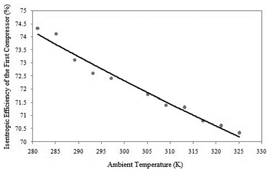
Variation in isentropic efficiency with the inlet air temperature of the first-stage compressor.

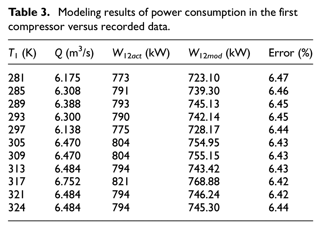
We can see some results of modeling of power consumption of the first compressor with recorded data in Table 3. The results showed a good agreement with the experimental data. In Mahshahr, the maximum and minimum ambient temperatures are so far from each other (1°C–48°C). The ambient temperature variations of this region are shown in Figure 3. These conditions lead to power consumption fluctuations of up to 14%.

Table 3.

Modeling results of power consumption in the first compressor versus recorded data.

T1 (K)	Q (m3/s)	W12act (kW)	W12mod (kW)	Error (%)
281	6.175	773	723.10	6.47
285	6.308	791	739.30	6.46
289	6.388	793	745.13	6.45
293	6.300	790	742.14	6.45
297	6.138	775	728.17	6.44
305	6.470	804	754.95	6.43
309	6.470	804	755.15	6.43
313	6.484	794	743.42	6.43
317	6.752	821	768.88	6.42
321	6.484	794	746.24	6.42
324	6.484	794	745.30	6.44

Figure 3.

Variations in the maximum and average temperatures of Mahshahr during a year. ²⁸

Figure 4 shows that ANN has an appropriate response to the variations of the selected parameters. There is an interesting reaction from ANN against a sudden change in the outlet air temperature from intercooler (according to Figure 4, we have a sudden change in the outlet air temperature after no. 100). This sudden change is caused by a change in operational parameters because of the change from winter season to summer season.

Figure 4.

Outlet air temperature from intercooler, comparison of ANN results with recorded data.

Table 4 shows some operational conditions of the intercooler. One can see from Table 4 that in different conditions, the decrease in air pressure is constant. Point that mass flow rate of inlet water is constant. Also, it is obvious from Table 5 that ANN has a good ability to predict the outlet air temperature from intercooler. According to Figure 5, the effectiveness of intercooler variation was from 0.7 to 1.1. It means that the inlet air temperature of the second compressor can be lower than that of the first compressor in a very hot condition. Therefore, the effectiveness can be >1 in some cases. This fact is not presented in the literature.

Table 4.

Operating conditions of the intercooler.

T2 (K)	T3 (K)	Tw,in (K)	Qin (m3/h)	ΔP (bar)
369	303	291	22,500	0.12
375	305	292	22,500	0.12
384	305	295	23,000	0.12
399	310	300	23,700	0.12
405	310	300	23,148	0.12
446	310	300	23,300	0.12

Table 5.

ANN performance in outlet air temperature prediction of the intercooler.

No. of tested data	Minimum error (K)	Maximum error (K)	Square mean error	Standard deviation
40	0.02	3.00	4.814	1.617

Figure 5.

Intercooler effectiveness variations against ambient temperature.

Also, a small variation in the inlet air temperature of the second compressor is an important point, and it means that the inlet air temperature range of this compressor is smaller than that of the first compressor because of the existence of intercooler.

Table 6 shows the comparison between modeling results and actual data of power consumption in the second compressor and the modeling error. The modeling error was in the range of the first compressor. Figure 6 shows the isentropic efficiency variation for the second compressor against the inlet air temperature. Isentropic efficiency variation for the second compressor was more limited because of narrow range of the inlet air temperature variation of the second compressor. In other words, the main reason for small variation in the inlet air temperature for the second compressor is small variation in cooling water temperature in summer and winter conditions. The maximum variation in power consumption of the second compressor was around 3% in summer condition when compared with winter condition.

Table 6.

Results of the second compressor power consumption modeling versus recorded data.

T3act (K)	T3model (K)	W34act (kW)	W34model (kW)	Error (%)
304	304.60	686	644.13	6.51
306	305.91	698	655.40	6.50
308	308.35	703	660.65	6.47
310	309.90	690	647.88	6.50
312	311.65	670	629.38	6.50
314	313.15	693	650.70	6.50
315	314.90	656	616.02	6.49

Figure 6.

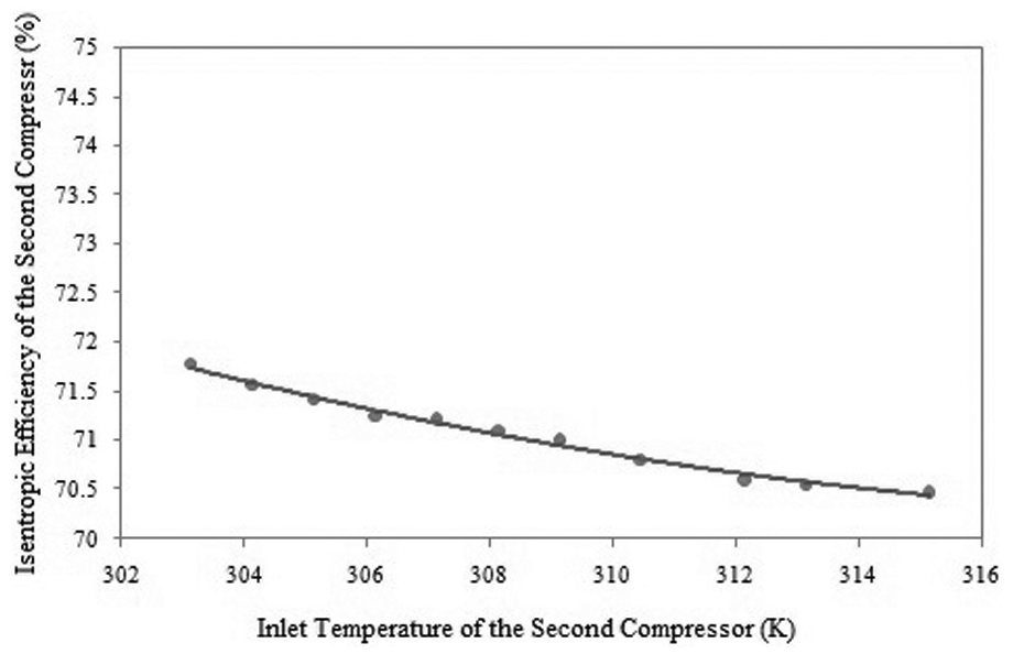
Isentropic efficiency variation for the second compressor versus inlet air temperature.

Optimization

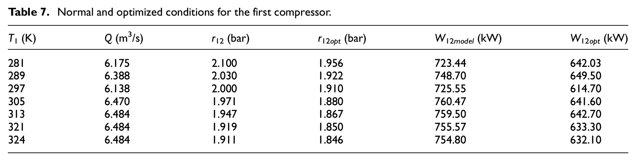
Operational conditions of the second compressor strongly depend on the operational condition of the first compressor and the intercooler. We presented optimized parameters for both compressors including pressure ratios and optimized power consumptions in Tables 7 and 8. The maximum optimization for power consumption of the first and second compressors was 20% and 6%, respectively. Also, minimum and maximum optimization for power consumption of the cycle was 2.9% and 9.6%, respectively.

Table 7.

Normal and optimized conditions for the first compressor.

T1 (K)	Q (m3/s)	r12 (bar)	r12opt (bar)	W12model (kW)	W12opt (kW)
281	6.175	2.100	1.956	723.44	642.03
289	6.388	2.030	1.922	748.70	649.50
297	6.138	2.000	1.910	725.55	614.70
305	6.470	1.971	1.880	760.47	641.60
313	6.484	1.947	1.867	759.50	642.70
321	6.484	1.919	1.850	755.57	633.30
324	6.484	1.911	1.846	754.80	632.10

Table 8.

Normal and optimized conditions for the second compressor.

T1 (K)	Q (m3/s)	r34 (bar)	r34opt (bar)	W34model (kW)	W34opt (kW)
281	6.175	1.180	1.943	650.79	693.75
289	6.388	1.180	1.911	653.00	685.14
297	6.138	1.180	1.895	611.80	630.03
305	6.470	1.782	1.876	625.98	636.40
313	6.484	1.776	1.855	647.12	660.20
321	6.484	1.776	1.848	614.43	621.34
324	6.484	1.776	1.845	608.74	612.00

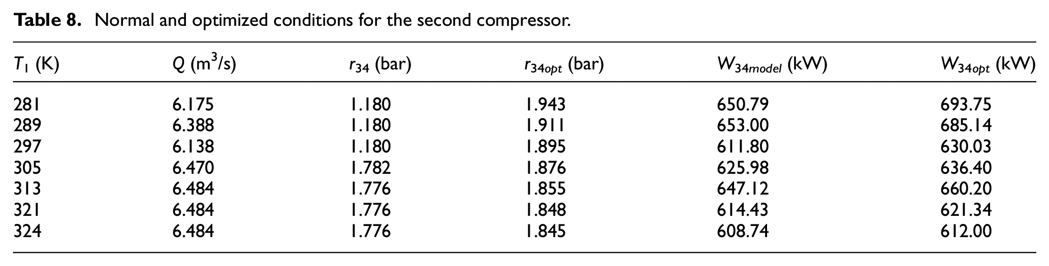
Figure 7 shows a comparison between outlet air temperature variations for the first compressor at normal and optimized conditions with regard to different inlet temperatures. It can be understood from Figure 7 that the outlet air temperature increases linearly with the increase in the inlet air temperature of the first compressor. At optimized condition, the outlet air temperature of the first compressor was around 10 K lower than the normal condition.

Figure 7.

Variations in the outlet air temperature from the first compressor at normal and optimized conditions.

Figure 8 shows specific work consumption of the first compressor versus inlet air temperature for both modeling and optimization conditions. In summer, the difference between normal and optimized conditions was increased in comparison with winter.

Figure 8.

Variations in specific work consumption of the first compressor as a function of the ambient temperature at normal and optimized conditions.

Using multistage compression system with an intercooler can tighten the range of temperature difference for all the compressors except the first one. Therefore, only the first compressor is affected with ambient temperature fluctuations because of the existence of intercooler. Figures 9 and 10 demonstrate the variations in the inlet and outlet air temperatures of the second compressor versus ambient temperature for modeling and optimization results.

Figure 9.

Variations in the inlet air temperature of the second compressor at normal and optimized conditions.

Figure 10.

Variations in the outlet air temperature from the second compressor at normal and optimized conditions.

As can be seen in Figure 9, despite ambient temperature increasing (and the increase in the inlet air temperature to intercooler), the inlet air temperature to the second compressor has same value in some points. The main reason for this phenomenon is intercooler effectiveness. Thermal performance of intercooler is a function of ambient temperature, cooling water temperature, and inlet air flow rate. According to Figures 9 and 10, one can observe that optimized results about outlet air temperature from the second compressor reduce sometimes with an increase in the ambient temperature. This is because of the difference in produced pressure ratios in the second compressor. In other words, the inlet air temperature to this compressor is equal in some points; however, the outlet air temperature varies because of the difference in optimized pressure ratios. Figures 11 and 12 demonstrate the variations in specific work consumption of the second compressor and total specific work of the cycle versus ambient air temperature, respectively.

Figure 11.

Variations in specific work consumption of the second compressor as a function of ambient temperature at normal and optimized conditions.

Figure 12.

Variations in total specific work versus ambient temperature at normal and optimized conditions.

It should be noted from Figure 12 that operating conditions and the cycle’s specific work consumption amounts are close to proportional modeling values at lower ambient temperature (in winter), although with a considerable increase in ambient temperature (in summer), the cycle keeps out from optimized conditions. Total specific work of the cycle reduces in the range of 2.8%–8.72% by compressor optimization in winter and summer conditions, respectively. This occurs due to small variations in optimized isentropic efficiency compared with actual operating efficiency.

Conclusion

According to the modeling and optimization methods, we can conclude that

• Our modeling method has a satisfactory level of accuracy for both compressors’ power consumptions.

• We used ANN to predict outlet air temperature from intercooler. It seems that this approach is preferred to the assumption of constant thermal effectiveness for intercooler.

• The cycle’s performance is too close to its optimum point in winter season. With a large increase in the ambient temperature (in summer), the cycle keeps away from optimum point. Total power of the cycle reduces in the range of 2.9%–9.6% by this optimization method in winter and summer conditions, respectively.

• To optimize total work of the cycle and to supply the required pressure ratio in the hot region, speed of compressors should be independent from each other. Consequently, compressor designing for a hot climate should be in the form of split shaft (especially the first-stage compressor) for operating compressors in different speeds and thus different pressure ratios to save more energy.

• To determine pressure ratios, one should consider intercooler performance. In winter season, pressure ratio of the first compressor should be larger than the other compressor (and vice versa in summer season), because in this condition, the inlet air temperature to the first compressor is smaller than that of the second compressor.