Petri net-based scheduling of time constrained single-arm cluster tools with wafer revisiting

Abstract

It is very difficult to schedule a single-arm cluster tool with wafer revisiting such that wafer residency time constraints are satisfied. This article conducts a study on this challenging problem for a single-arm cluster tool with atomic layer deposition process. With a so-called p-backward strategy being applied, a Petri net model is developed to describe the dynamic behavior of the system. Based on the model, the existence of a feasible schedule is analyzed, schedulability conditions are derived, and scheduling algorithms are presented if there is a schedule. A schedule is obtained by simply setting the robot waiting time if schedulable, and it is very computationally efficient. The obtained schedule is shown to be optimal. Illustrative examples are given to demonstrate the proposed approach.

Introduction

In semiconductor manufacturing, cluster tools that adopt single-wafer processing technology are widely used in wafer processing for better quality control and lead time reduction. A typical cluster tool is configured with several process modules (PMs), a wafer handling robot, and two loadlocks for wafer loading and unloading. According to the number of arms equipped for the robot, a cluster tool is called a single-arm or dual-arm cluster tool as shown in Figure 1.

Figure 1.

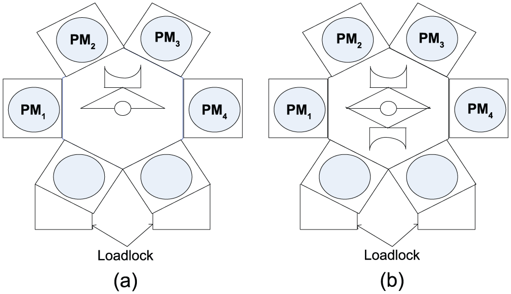
Cluster tools: (a) single-arm robot and (b) dual-arm robot.

With two loadlocks, a cluster tool can operate uninterruptedly under steady state. Under the steady state, extensive studies have been done for modeling, performance evaluation, and scheduling of both cluster tools^1–7 and multi-cluster tools.^8–13 Under the steady state, if wafer processing time dominates the process, then a cluster tool is called to be process-bound, while it is called to be transport-bound if the robot is always busy. According to Kim et al., ¹⁴ the time taken for the robot to move from one step to another can be treated as the same and is much shorter than the wafer processing time. In this case, a cluster tool operates in the process-bound region such that a backward scheduling strategy is optimal for a single-arm tool^15,16 and a swap scheduling strategy is optimal for a dual-arm tool. ⁵

The afore-mentioned studies are conducted under the assumption that there is no constraint on the wafer sojourn time in a PM. For some wafer fabrication processes, such as low-pressure chemical-vapor deposition, there are strict wafer residency time constraints which require that a wafer should be removed from a PM within a given time after it is processed.^14,17–23 Without any intermediate buffer between the PMs, the scheduling problem of cluster tools with residency time constraints is very complex and challenging. The scheduling problem of cluster tools with wafer residency time constraints is studied and techniques are developed to find an optimal periodical schedule.^14,17 To improve computational efficiency, this problem is further tackled for both single-arm and dual-arm cluster tools using schedulability analysis and closed-form solution methods are presented.^24,25 They present a so-called robot waiting method. By this method, a schedule is parameterized by robot waiting time and can be obtained by setting the robot waiting time.

The above-mentioned work is done for wafer fabrication processes with no wafer revisiting. Some wafer fabrication processes, such as the atomic layer deposition (ALD) process, require that a wafer should be processed by some processing steps more than once, leading to a revisiting process.^26–31 With wafer revisiting, a cluster tool is no longer a flow-shop and methods developed for scheduling tools without wafer revisiting are not applicable. As shown in Wu et al., ²⁶ for a dual-arm cluster tool with wafer revisiting, a three-wafer cyclic schedule is obtained if a swap strategy is applied and the system may never reach a steady state. Furthermore, with wafer revisiting, a cluster tool is deadlock-prone, which further complicates the scheduling problem of a cluster tool. Lee and Lee ²⁸ pioneer the study of scheduling single-arm cluster tools with wafer revisiting. They model the system by a Petri net (PN) and the scheduling problem is then formulated as a mixed integer programming to find an optimal periodical schedule. Following the work in Lee and Lee, ²⁸ Wu et al. ²⁹ develop a maximally permissive deadlock-avoidance policy for a single-arm cluster tool with the ALD process. Based on the model and the control policy, it is shown that, to find an optimal schedule, one needs to examine several schedules only. Based on this finding, analytical expressions are proposed to find the optimal schedule by selecting the best one from these schedules. For dual-arm cluster tools with wafer revisiting, a method is presented to obtain a two-wafer cyclic schedule that is better than a three-wafer schedule. ²⁷ Since a one-wafer cyclic schedule is easy to implement and control, this problem is further investigated and a modified swap strategy is proposed to obtain a one-wafer periodical schedule. ³⁰ It is shown that such a schedule can reach the lower bound of cycle time. The scheduling problem of dual-arm cluster tools with both wafer revisiting and residency time constraints is studied and effective techniques are proposed to find an optimal one-wafer cyclic schedule. ³¹

However, to the best knowledge of the authors, up to now, no study has been done on the scheduling problem of single-arm cluster tools with both wafer revisiting and wafer residency time constraints. Note that it is more difficult to avoid deadlock for a single-arm cluster tool with wafer revisiting than for a dual-arm tool. Thus, scheduling single-arm cluster tools with both wafer revisiting and wafer residency time constraints is more complicated. The aim of this work is to cope with this challenging problem for a single-arm cluster tool. The problem is modeled by a PN using a p-backward strategy explained later. With the model, analysis on the existence of a feasible schedule is carried out and conditions under which a schedule exists are presented. If it is schedulable, a schedule is very efficiently obtained by simply setting the robot waiting time. The obtained schedule is shown to be optimal in terms of cycle time.

In the next section, we develop the PN model for the system. Based on it, Section “System scheduling” carries out the schedulability analysis, establishes the schedulability conditions, and presents scheduling algorithms to obtain the optimal schedule. Then, in the following section, illustrative examples are used to demonstrate the proposed method. Finally, Section “Conclusion” concludes this work.

Modeling by PN

PNs are recognized as a powerful tool for dealing with concurrent activities and resource allocation. They are widely used for modeling, analysis, and control of manufacturing systems.^32–38 This work adopts PN to model the dynamic behavior of a single-arm cluster tool with both wafer residency time constraints and wafer revisiting.

Finite capacity PN

Scheduling a cluster tool is to effectively allocate its limited resources to tasks. To do so, this work adopts the resource-oriented PN (ROPN)^39–42 to model the system. It is a finite capacity PN and its basic concept is based on Wu and Zhou ⁴² and Murata. ⁴³ It is denoted as PN = (P, T, I, O, M, K), where P and T are finite sets of places and transitions with P∩T = ∅ and P∪T ≠ ∅; I: P × T → ℕ = {0, 1, 2, …} and O: P × T → ℕ describe the relation from P to T and T to P, respectively; M: P → ℕ is a marking with M(p) being the number of tokens in place p and M₀ being the initial marking; K: P → {1, 2, 3, …} is a capacity function with K(p) representing the maximum number of tokens that can be held by p at a time.

Let ^•t = {p: p ∈ P and I(p, t) > 0} be the pre-set of transition t and t^• = {p: p ∈ P and O(p, t) > 0} be its post-set. Similarly, p’s pre-set ^•p = {t ∈ T: O(p, t) > 0} and post-set p^• = {t ∈ T: I(p, t) > 0}. Then, the transition enabling and firing rules are defined as follows.

Definition 2.1

A transition t ∈ T in a finite capacity PN is said to be enabled if the following conditions are satisfied

$$M(p)\ge I(p,t),\forall p\in P$$

(1)

and

$$K(p)\ge M(p)-I(p,t)+O(p,t),\forall p\in P$$

(2)

By Definition 2.1, when Condition (1) is met, t is said to be process-enabled, and while Condition (2) is met, t is said to be resource-enabled. Thus, t is enabled if it is both process- and resource-enabled.

An enabled t ∈ T at marking M can fire. The firing of t transforms the PN from M to M′ according to

$$M\prime (p)=M(p)-I(p,t)+O(p,t),\forall p\in P$$

(3)

Modeling activity sequences

In wafer fabrication, ALD is a typical revisiting process and, as done in Wu et al., ²⁹ this work focuses on the ALD process. In an ALD, a wafer visits Step 1 first and then it goes to Steps 2 and 3 sequentially for processing. After being processed by Step 3, it goes back to Steps 2 and 3. This process is repeated for several times. To control the quality, every time the wafer visits Steps 2 and 3, the exactly same processing environment is required. To ensure the processing environment requirement, each step is configured with only one PM. We assume that PM _i is configured for Step i. Thus, as presented in Wu et al., ²⁹ the wafer flow pattern for this process can be denoted as (PM₁, (PM₂, PM₃) ^h , PM₄) with (PM₂, PM₃) ^h being the revisiting process and h ≥ 2. For the simplicity of presentation, this work focuses on the case when h = 2. Note that the obtained results with h = 2 can be extended to cases with h > 2. Then, a single-arm cluster tool with both wafer residency time constraints and wafer revisiting is modeled by an ROPN as follows.

Let ℕ _n  = {1, 2, 3,…, n} and Ω _n  = ℕ _n ∪{0}. As shown in Figure 2, timed place p_n, n ∈ ℕ₄, models the PM for Step n with K(p_n) = 1 representing that there is only one PM. The loadlocks are treated as a processing step with processing time being zero. They are modeled by p₀ with K(p₀) = ∞ representing that the loadlocks can hold all wafers in a tool. Timed place q_n2 with K(q_n2) = 1, n ∈ Ω₄, models the robot waiting before unloading a wafer from p_n. Non-timed places q_n1 and q_n3 with K(q_n1) = K(q_n3) = 1, n ∈ Ω₄, are used to connect two neighboring steps. Place r with K(r) = 1 models the robot (R). When M(r) = 1, the robot is idle and ready for performing a task.

Figure 2.

PN model for the system with wafer flow pattern (PM₁, (PM₂, PM₃) ^h , PM₄).

With the resources in the system being modeled, transitions are used to model the material flows. Timed transition t_ij, i, j ∈ Ω₄, models the activity for the robot moving from p_i to p_j with a wafer being carried. Timed transition y_ij, i, j ∈ Ω₄, models the activity for the robot moving from p_i to p_j without carrying a wafer. Transitions s_n1 and s_n2 represent the loading and unloading of a wafer into and from p_n, n ∈ Ω₄, respectively. By doing so, the structure of the model is formed.

With the developed PN structure, by putting a V-token representing a virtual wafer, the initial marking M₀ is set as follows. Set M₀(p_i) = 1, i ∈ ℕ₄\{1}, M₀(p₁) = 0, and M₀(p₀) = n to indicate that there are always wafers in the loadlocks to be processed; M₀(r) = 0; M₀(q_ij) = 0, i ∈ N₄ and j ∈ Ω₃, and M₀(q₀₂) = 1, indicating that the robot is waiting at the loadlocks for unloading a wafer there.

With wafer revisiting process, there are two ways for a token in q₃₃ to go, one is to q₂₁ by firing t₃₂ and the other is to q₄₁ by firing t₃₄, leading to a conflict. To eliminate such a conflict, colors are introduced to the model to form a colored PN as follows.

Definition 2.2

Transition t_i in the PN is defined to have a unique color C(t_i) = c_i.

By Definition 2.2, the colors of t₃₂ and t₃₄ are c₃₂ and c₃₄, respectively. Let W_d(g) be the dth wafer released into the system and being processed for the gth time by a PM. Then, we can define the color of a token as follows.

Definition 2.3

Define the color of a token W_d in q₃₃ as C(q₃₃, W_d) = c_3j if it will go to Step j for processing when it leaves q₃₃.

By Definition 2.3, we have C(q₃₃, W_d(q)) =C(t₃₂) = c₃₂, 1 ≤ q < h, and (q₃₃, W_d(h)) = C(t₃₄)= c₃₄. Note that in the model, only q₃₃ has multiple output transitions. Hence, by Definitions 2.2 and 2.3, conflict is eliminated. Besides conflict, deadlock is an important issue for operating a single-arm tool with wafer revisiting. To avoid deadlock, we present a control policy by the following definition.

Definition 2.4

At any marking M, transition y₂₀ is control-enabled only if the transition firing sequence t₁₂ → s₂₁ has just been performed; y₀₃ is control-enabled only if s₀₁ has just fired; y₁₄ is control-enabled only if s₁₁ has just fired; y₄₂ is control-enabled only if s₄₁ has just fired; y₂₂ is control-enabled only if the transition firing sequence t₃₂ → s₂₁ has just been performed; y₃₃ is control-enabled only if the transition firing sequence y₄₂ → s₂₂ → t₂₃ → s₃₁ has just been performed; and y₃₁ is enabled only if the transition firing sequence t₃₂ → s₂₁ → y₂₂ → s₂₂ → t₂₃ → s₃₁ has just been performed.

Let M = (S₁, S₂, S₃, S₄) represent the marking of the system, where S_i represents the state at Step i, i ∈ ℕ₄. S_i = {W_d(g)} represents that the dth wafer is being processed at Step i for the gth time, or {V_d(g)} represents that the dth virtual wafer is being processed at Step i for the gth time, and {null} represents that Step i is idle. In this way, as above discussed, we have M₀ = ({null}, {V₃(1)}, {V₂(2)}, {V₁(1)}). Then, by Definition 2.4, at M₀, the only enabled transition is s₀₂. After s₀₂ fires, R performs task sequence 〈t₀₁ → s₁₁ → y₁₄ → s₄₂ → t₄₀ → s₀₁ → y₀₃ → s₃₂ → t₃₄ (according to its color) → s₄₁ → y₄₂ → s₂₂ → t₂₃ → s₃₁ → y₃₃ → waiting for the completion of the wafer at Step 3 → s₃₂ → t₃₂ (according to its color) → s₂₁ → y₂₂ → waiting for the completion of the wafer at Step 2 → s₂₂ → t₂₃ → s₃₁ → y₃₁ → s₁₂ → t₁₂ → s₂₁ → y₂₀ → s₀₂〉 such that a cycle is completed and there is no deadlock. This implies that by the control policy given in Definition 2.4, the model is deadlock-free. It can be verified that this control policy is maximally permissive, that is, it restricts no permissive state.

Task time modeling

In order to schedule the process, it is necessary to model the time taken for performing each activity. From the PN model, both transitions and places represent tasks that take time. As done in Lee and Lee ²⁸ and Wu et al., ²⁹ we assume that the time taken for each activity is deterministic and known. The time taken for the robot to move from Steps i to j, i ≠ j, with or without holding a wafer is assumed to be same ¹⁴ and denoted by µ, that is, it takes µ time units to fire t_ij and y_ij. Note that in the revisiting process, after loading a wafer into p₃/p₂, the robot waits there for the completion of the wafer and it does nothing and takes no time. Similarly, the time taken for the robot to unload (firing s_i2)/load (firing s_i1), a wafer from/into a step is assumed to be the same as well and it is denoted by λ. The time taken for processing a wafer in p_i, i ∈ Ω₄, is α_i with α_i > 0, i ≠ 0, and α₀ = 0.

Let δ_i be the longest time for which a wafer can stay in a PM at Step i without being scrapped after being processed. Then, with wafer residency time constraints, the wafer sojourn time at Step i should be within [α_i, α_i+δ_i], that is, a token should stay in PM _i for at least α_i time units and no more than α_i+δ_i time units. We use τ₁ and τ₄ to denote the wafer sojourn time at Steps 1 and 4, respectively; and τ_2j and τ_3j, j ∈ N₂ to denote the wafer sojourn time for the jth visiting Steps 2 and 3, respectively. Note that no wafer residency time constraint is imposed on Step 0. The symbols and explanation are summarized in Table 1.

Table 1.

Time durations associated with transitions and places.

Symbol	Transition or place	Actions	Allowed time duration
λ	si 1  ∈ T	Robot loads a wafer into Step i, i ∈ Ω 4	λ
λ	si 2  ∈ T	Robot unloads a wafer from Step i, i ∈ Ω4	λ
µ	tij ∈ T	Robot moves from Steps i to j with a wafer carried, i, j ∈ Ω4	µ
µ	yij ∈ T	Robot moves from Steps i to j without carrying a wafer, i, j ∈ Ω4	µ, i ≠ j; otherwise, 0
τ 1 and τ4	p 1 and p4 ∈ P	A wafer is being processed and waiting in p1 and p4	τ 1  ∈ [α1, α1+δ1] τ4 ∈ [α4, α4+δ4]
τ 2j and τ3j	p 2 and p3 ∈ P	A wafer being processed and waiting in p2 and p3 for the jth time, j ∈ ℕ2	τ 2 j ∈ [α2, α2+δ2] and τ3j ∈ [α3, α3+δ3], j ∈ ℕ2
ωi	qi 2  ∈ P	Robot waits before unloading a wafer from PM i , i ∈ Ω4	≥0
ωi	qi 3  ∈ P	Robot waits after unloading a wafer from PM i , i ∈ Ω4	0
ωi	qi 1  ∈ P	Robot waits before loading a wafer from PM i , i ∈ Ω4	0

From the above analysis, for a single-arm cluster tool with wafer revisiting and residency time constraints, according to Wu et al.^24,29 we have the following schedulability definition.

Definition 2.5

Given the wafer sojourn time interval [α_i, α_i+δ_i] for Step i, i ∈ ℕ₄, if there exists a schedule such that whenever s_i2, i ∈ {1, 4}, fires, α_i ≤ τ _i  ≤ α_i+δ_i holds, and whenever s_i2 fires, α_i ≤ τ_ij ≤ α_i+δ_i, i ∈ {2, 3} and j ∈ ℕ₂, holds, then a single-arm cluster tool with wafer revisiting and residency time constraints is schedulable.^24,29 With the PN model, we discuss the scheduling problem next.

System scheduling

In Wu et al., ²⁹ a p-backward strategy is proposed to schedule a single-arm cluster tool for the ALD process without taking wafer residency time constrains into account. Based on the PN model, this work adopts this strategy to explore the schedulability and scheduling problem of a single-arm cluster tool with residency time constraints for the ALD process. If schedulable, efficient algorithm is developed to find an optimal schedule.

P-backward scheduling

To make the scheduling analysis, we need to present the p-backward scheduling strategy for a single-arm cluster tool with wafer revisiting. Based on the PN model, we show how a p-backward strategy works. Since a single-arm cluster tool with wafer revisiting is deadlock-prone, to avoid deadlock, the system must start from a proper state. We assume that the system starts from marking M₁ = ({null}, {W₃(1)}, {W₂(2)}, {W₁(1)}) and, at the same time, the robot is idle, or M₁(r) = 1. Note that this marking is consistence with M₀ that is set in the last section and can be reached by applying a p-backward strategy. By starting from M₁ with a p-backward strategy being applied, the system evolves as follows.

• Step 1: Transition firing sequence σ₁ = 〈firing y₂₀ → s₀₂ → t₀₁ → s₁₁〉 (the robot goes to the loadlocks from PM₂ → waits in q₀₂ → unloads W₄ there → moves to PM₁ → loads W₄ into PM₁) is performed such that W₄(1) is put into Step 1. By doing so, it transforms the system from M₁ to M₂ = ({W₄(1)}, {W₃(1)}, {W₂(2}, {W₁(1)}).

• Step 2: Transition firing sequence σ₂ = 〈firing y₁₄ → waiting in q₄₂ → s₄₂ → t₄₀ → s₀₁〉 (the robot goes to PM₄ from PM₁ → waits in q₄₂ → unloads W₁ there → moves to the loadlocks → loads W₁ into the loadlocks) is performed such that M₃ = ({W₄(1)}, {W₃(1)}, {W₂(2)}, {null}) is reached.

• Step 3: Transition firing sequence σ₃ = 〈firing y₀₃ → waiting in q₃₂ → s₃₂ → t₃₄ → s₄₁〉 (the robot goes to PM₃ from the loadlocks → waits in q₃₂ → unloads W₂ there → moves to PM₄ → loads W₂ into PM₄) is performed such that M₄ = ({W₄(1)}, {W₃(1)}, {null}, {W₂(1)}) is reached.

• Step 4: Transition firing sequence σ₄ = 〈firing y₄₂ → waiting in q₂₂ → s₂₂ → t₂₃ → s₃₁〉 (the robot goes to PM₂ from PM₄ → waits in q₂₂ → unloads W₃ there → moves to PM₃ → loads W₃ into PM₃) is performed such that M₅ = ({W₄(1)}, {null}, {W₃(1)}, {W₂(1)}) is reached.

• Step 5: Transition firing sequence σ₅ = 〈firing y₃₃ → waiting q₃₂ → s₃₂ → t₃₂ → s₂₁〉 (the robot stays at PM₃ → waits in q₃₂ → unloads W₃ there → moves to PM₂ → loads W₃ into PM₂) is performed such that M₆ = ({W₄(1)}, {W₃(2)}, {null}, {W₂(1)}) is reached.

• Step 6: Transition firing sequence σ₆ = 〈firing y₂₂ → waiting q₂₂ → s₂₂ → t₂₃ → s₃₁〉 (the robot stays at PM₂ → waits in q₂₂ → unloads W₃ there → moves to PM₃ → loads W₃ into PM₃) is performed such that M₇ = ({W₄(1)}, {null}, {W₃(2)}, {W₂(1)}) is reached.

• Step 7: Transition firing sequence σ₇ = 〈firing y₃₁ → waiting in q₁₂ → s₁₂ → t₁₂ → s₂₁〉 (the robot goes to PM₁ from PM₃ → waits in q₁₂ → unloads W₄ there → moves to PM₂ → loads W₄ into PM₂) is performed such that M₈ = ({null}, {W₄(1)}, {W₃(2)}, {W₂(1)}) is reached.

Note that marking M₈ is equivalent to M₁ in the sense of dynamic behavior of PN. Hence, by transforming M₁ to M₈, a cycle is completed. This is what a p-backward strategy does. With the PN model, it is easy to understand the scheduling strategy.

Cycle time analysis

With the above discussion, we can analyze the cycle time for the system. Let φ_j be the time taken for the robot to perform σ_j, j ∈ ℕ₇. Then, from the time modeling, we have φ₁ = µ+ω₀+λ+µ+λ = 2µ+2λ+ω₀. Similarly, for σ_2–7, we have φ₂ = 2µ+2λ+ω₄; φ₃ = 2µ+2λ+ω₃; φ₄ = 2µ+2λ+ω₂; φ₅ = µ+2λ+α₃; φ₆ = µ+2λ+α₂; and φ₇ =2µ+2λ+ω₁.

Since σ_1–7 form a robot cycle, the robot cycle time is as follows

$$\eta ={\displaystyle \sum _{i=1}^7{\phi }_i}=(14\lambda +12\mu +{\alpha }_2+{\alpha }_3)+{\displaystyle \sum _{i=0}^4{\omega }_i}={\eta }_1+{\eta }_2$$

(4)

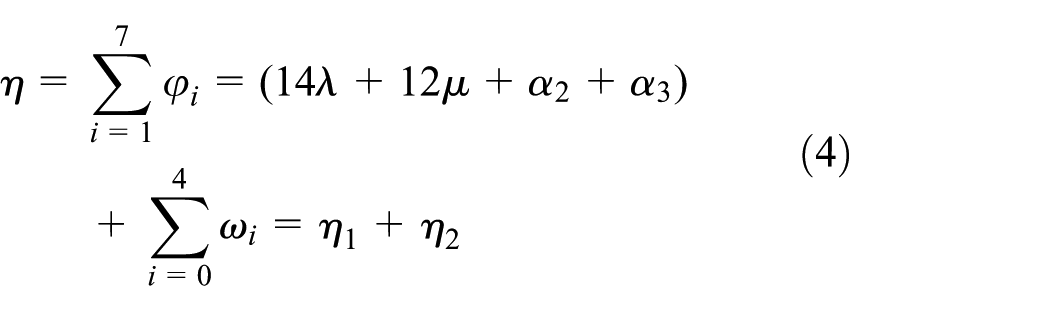
where η₁ = 14λ+12µ+α₂+α₃ is the robot task time in a cycle and ${\eta }_2=\sum _{i=0}^4{\omega }_i$ is the robot waiting time in a cycle. Note that η₁ is constant and known in advance and ω_0–4 in η₂ should be determined by a schedule.

Based on the fact that the cycle time of the entire system must be equal to the robot cycle time, ²⁴ with the robot cycle time obtained, we can analyze the wafer sojourn time at each step. It follows from the above analysis that the wafer sojourn time at Step 1 is equal to the robot cycle time minus the time taken for performing σ₁ and the time for firing s₁₂, t₁₂, and s₂₁ in σ₇, that is, we have

$${\tau }_1=\eta -(2\mu +2\lambda +{\omega }_0)-(\mu +2\lambda )=\eta -3\mu -4\lambda -{\omega }_0$$

(5)

Similarly, for Step 4, we have

$${\tau }_4=\eta -3\mu -4\lambda -{\omega }_3$$

(6)

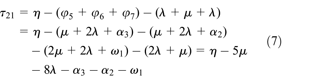
For Step 2, the sojourn time taken for a wafer to visit the step for the first time is different from that for a wafer to visit the step for the second time. We use τ₂₁ and τ₂₂ to denote them, respectively. It follows from the above transition firing analysis that τ₂₁ is equal to the robot cycle time minus the time taken for σ_5–7 and the time taken for firing s₂₂, t₂₃, and s₃₁ in σ₄. Thus, we have

$$\begin{array}{cc}\multicolumn{1}{c}{{\tau }_{21}}& =\eta -({\phi }_5+{\phi }_6+{\phi }_7)-(\lambda +\mu +\lambda )\hfill \\ \multicolumn{1}{c}{}& =\eta -(\mu +2\lambda +{\alpha }_3)-(\mu +2\lambda +{\alpha }_2)\hfill \\ \multicolumn{1}{c}{}& -(2\mu +2\lambda +{\omega }_1)-(2\lambda +\mu )=\eta -5\mu \hfill \\ \multicolumn{1}{c}{}& -8\lambda -{\alpha }_3-{\alpha }_2-{\omega }_1\hfill \end{array}$$

(7)

When a wafer visits Step 2 for the second time, the robot loads it into PM₂ and waits here for its completion. Thus, we have

$${\tau }_{22}={\alpha }_2$$

(8)

Similarly, we can calculate the wafer sojourn time for Step 3 and we have

$${\tau }_{31}={\alpha }_3$$

(9)

$${\tau }_{32}=\eta -5\mu -8\lambda -{\alpha }_3-{\alpha }_2-{\omega }_2$$

(10)

With wafer residency time constraints, to make a schedule feasible, the cycle time for each step should be in a permissive range. Thus, we analyze such a range for each step as follows. For Step 1, it follows from the above analysis that to complete a wafer requires three robot moving tasks between steps (t₀₁, t₁₂, and y₂₁), two wafer unloading tasks (s₀₂ and s₁₂), and two wafer loading tasks (s₁₁ and s₂₁). Thus, with the wafer staying time in Step 1, the time taken for this process is as follows

$${\theta }_1={\tau }_1+3\mu +4\lambda +{\omega }_0$$

(11)

To be feasible, we have τ₁ ∈ [α₁, α₁+δ₁]. Hence, the permissive shortest cycle time at Step 1 is as follows

$${\theta }_{1S}={\alpha }_1+3\mu +4\lambda +{\omega }_0$$

(12)

and the permissive longest cycle time at Step 1 is as follows

$${\theta }_{1L}={\alpha }_1+{\delta }_1+3\mu +4\lambda +{\omega }_0$$

(13)

Similarly, the cycle time for completing a wafer at Step 4 is as follows

$${\theta }_4={\tau }_4+3\mu +4\lambda +{\omega }_3$$

(14)

The permissive shortest cycle at Step 4 is as follows

$${\theta }_{4S}={\alpha }_4+3\mu +4\lambda +{\omega }_3$$

(15)

and the permissive longest cycle time at Step 4 is as follows

$${\theta }_{4L}={\alpha }_4+{\delta }_4+3\mu +4\lambda +{\omega }_3$$

(16)

For Step 2 in the revisiting process, we analyze the wafer cycle as follows. By firing s₂₁ (σ₈ = 〈s₂₁ (λ)〉), a wafer is loaded into Step 2 for processing for the first time, which is followed by transition firing sequence σ₉ = 〈y₂₀ → s₀₂ → t₀₁ → s₁₁ → y₁₄ → s₄₂ → t₄₀ → s₀₁ → y₀₃ → s₃₂ → t₃₄ → s₄₁ → y₄₂〉. During the time for performing σ₉, the wafer just loaded into Step 2 is being processed. Hence, the time taken for performing σ₉ is the wafer sojourn time for the first visiting Step 2, that is, τ₂₁. Then, transition firing sequence σ₁₀ = 〈t₂₃ (µ) → s₃₁ (λ) → y₃₃ (0) → waiting for the completion at Step 3 (α₃) → s₃₂ (λ) → t₃₂ (µ) → s₂₁ (λ) (loading the wafer into Step 2 to be processed for the second time) → y₂₂ (0) → waiting for the completion of the wafer at Step 2 (τ₂₂) → s₂₂ (λ) → t₂₃ (µ) → s₃₁ (λ) → y₃₁ (µ) → waiting in q₁₂ (ω₁) → s₁₂ (λ) → t₁₂ (µ)〉 is performed. By performing σ_8–10, a cycle is completed at Step 2. Thus, the time taken for completing a wafer at Step 2 is as follows

$${\theta }_2={\tau }_{21}+{\tau }_{22}+{\alpha }_3+5\mu +8\lambda +{\omega }_1$$

(17)

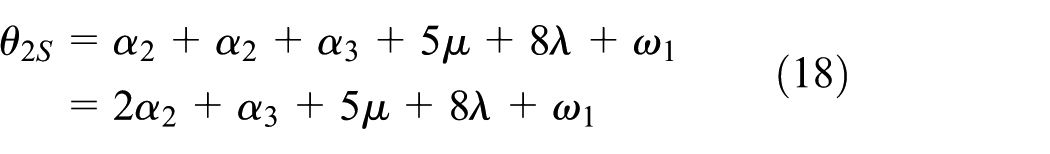
With τ₂₁ ∈ [α₂, α₂+δ₂] and τ₂₂ = α₂, the permissive shortest cycle at Step 2 is as follows

$${\theta }_{2S}={\alpha }_2+{\alpha }_2+{\alpha }_3+5\mu +8\lambda +{\omega }_1=2{\alpha }_2+{\alpha }_3+5\mu +8\lambda +{\omega }_1$$

(18)

and the permissive longest cycle time at Step 2 is as follows

$${\theta }_{2L}={\alpha }_2+{\delta }_2+{\alpha }_2+{\alpha }_3+5\mu +8\lambda +{\omega }_1=2{\alpha }_2+{\delta }_2+{\alpha }_3+5\mu +8\lambda +{\omega }_1$$

(19)

For Step 3, similar to Step 2, we analyze the process as follows. We have the following transition firing sequence σ₁₁ = 〈s₃₁ (a wafer is loaded into Step 3 to be processed for the first time, λ) → y₃₃ (0) → waiting for the completion of the wafer at Step 3 (τ₃₁) → s₃₂ (λ) → t₃₂ (µ) → s₂₁ (λ) → y₂₂ (0) → waiting for the completion of the wafer at Step 2 (α₂) → s₂₂ (λ) → t₂₃ (µ) → s₃₁ (λ)〉. Then, transition firing sequence σ₁₂ = 〈y₃₁ → s₁₂ → t₁₂ → s₂₁ → y₂₀ → s₀₂ → t₀₁ → s₁₁ → y₁₄ → s₄₂ → t₄₀ → s₀₁ → y₀₃〉 is performed. During the time for performing σ₁₂, a wafer for its second visiting of Step 3 is completed. Thus, the time taken for doing so is τ₃₂. Finally, to complete a cycle, transition firing sequence σ₁₃ = 〈s₃₂ (λ) → t₃₄ (µ) → s₄₁ (λ) → y₄₂ (µ) → waiting in q₂₂ (ω₂) → s₂₂ (λ) → t₂₃ (µ)〉 is performed. Thus, the cycle time for Step 3 is as follows

$${\theta }_3={\tau }_{31}+{\tau }_{32}+{\alpha }_2+5\mu +8\lambda +{\omega }_2$$

(20)

With τ₃₁ = α₃ and τ₃₂ ∈ [α₃, α₃+δ₃], the permissive shortest cycle at Step 3 is as follows

$${\theta }_{3S}=2{\alpha }_3+{\alpha }_2+5\mu +8\lambda +{\omega }_2$$

(21)

and the permissive longest cycle time at Step 3 is as follows

$${\theta }_{3L}=2{\alpha }_3+{\delta }_3+{\alpha }_2+5\mu +8\lambda +{\omega }_2$$

(22)

With the above timeliness analysis, we discuss the scheduling problem next. Note that the above-derived expressions are functions of robot waiting time. Hence, the scheduling problem is to decide the robot waiting time ω_i’s to obtain a schedule if it exists.

Schedulability and scheduling algorithm

Let θ be the production cycle time of the system. Then, the production cycle time for all the steps must be θ. Also, the robot cycle time should be equal to the production cycle time too, that is, we have

$$\theta ={\theta }_1={\theta }_2={\theta }_3={\theta }_4=\eta$$

(23)

Based on the above analysis, to make equation (23) hold, we need to decide ω_i’s in η₂. Also, to schedule a cluster tool, the production rate should be maximized, which requires to minimize η₂. Furthermore, with wafer residency time constraints, schedule feasibility is essential. To be feasible, a schedule should ensure that θ_i is in an acceptable interval. Let π_iL and π_iU denote the lower and upper bounds of θ_i. It follows from the above analysis that when ω₀ = ω₁ = ω₂ = ω₃ = ω₄ = 0, θ_iS and θ_iL are the lower and upper bounds of θ_i, respectively. Thus, by removing the robot waiting time from equations (12), (13), (15), (16), (18), (19), (21), and (22), we have the following lower and upper bounds of θ_i

$${\pi }_{1L}={\alpha }_1+3\mu +4\lambda$$

(24)

$${\pi }_{1U}={\alpha }_1+{\delta }_1+3\mu +4\lambda$$

(25)

$${\pi }_{2L}=2{\alpha }_2+{\alpha }_3+5\mu +8\lambda$$

(26)

$${\pi }_{2U}=2{\alpha }_2+{\delta }_2+{\alpha }_3+5\mu +8\lambda$$

(27)

$${\pi }_{3L}=2{\alpha }_3+{\alpha }_2+5\mu +8\lambda$$

(28)

$${\pi }_{3U}=2{\alpha }_3+{\delta }_3+{\alpha }_2+5\mu +8\lambda$$

(29)

$${\pi }_{4L}={\alpha }_4+3\mu +4\lambda$$

(30)

$${\pi }_{4U}={\alpha }_4+{\delta }_4+3\mu +4\lambda$$

(31)

Let π_Lmax = max{π_iL, i ∈ ℕ₄} and π_Umin = min{π_iU, i ∈ ℕ₄}, we have the following lemma.

Lemma 1

If η₁ > π_Umin, the system is not schedulable.

Proof

It follows from the above discussion that θ = η ≥ η₁. When η = η₁, we have ω₀ = ω₁ = ω₂ = ω₃ = ω₄ = 0. In this case, if π_Umin = π_kU, k ∈ {1, 4}, by equations (5) and (6), we have τ_k = η₁ − 3µ − 4λ > π_kU − 3µ − 4λ = α_k+δ_k+3µ+4λ − 3µ − 4λ = α_k+δ_k. This implies that the wafer residency time constraints are violated for Step k, k ∈ {1, 4}. If π_Umin = π_2U, by equation (7), we have τ₂₁ = η₁ − 5µ − 8λ − α₃ − α₂ > π_2U − 5µ − 8λ − α₃ − α₂ = 2α₂+δ₂+α₃+5µ+8λ − 5µ − 8λ − α₃ − α₂ = α₂+δ₂. Hence, the wafer residency time constraints are violated for Step 2. If π_Umin = π_3U, by equation (7), we have τ₃₂ = η₁ − 5µ − 8λ − α₃ − α₂ > π_3U − 5µ − 8λ − α₃ − α₂ = 2α₃+δ₃+α₂+5µ+8λ − 5µ − 8λ − α₃ − α₂ = α₃+δ₃. The wafer residency time constraints are violated for Step 3.

Then, we discuss the case when η > η₁. In this case, we have ${\eta }_2=\eta -{\eta }_1=\sum _{i=0}^4{\omega }_i$ and ω_i ≤ η − η₁, ∀i ∈ Ω₄. If π_Umin = π_kU, k ∈ {1, 4}, by equations (5) and (6), we have τ_k = η − 3µ − 4λ − ω_k − 1 ≥ η − 3µ − 4λ − (η − η₁) = η₁ − 3µ − 4λ > π_kU − 3µ − 4λ = α_k+δ_k+3µ+4λ − 3µ − 4λ = α_k+δ_k. The residency time constraints are violated for Step k, k ∈ {1, 4}. If π_Umin = π_2U, by equation (7), we have τ₂₁ =η − 5µ − 8λ − α₃ − α₂ − ω₁ ≥ η − 5µ − 8λ − α₃ − α₂ − (η − η₁) = η₁ − 5µ − 8λ − α₃ − α₂ > π_2U − 5µ − 8λ − α₃ − α₂ = 2α₂+δ₂+α₃+5µ+8λ − 5µ − 8λ − α₃ − α₂ = α₂+δ₂. The residency time constraints are violated for Step 2. If π_Umin = π_3U, by equation (10), we have τ₃₂ = η − 5µ − 8λ − α₃ − α₂ − ω₂ ≥ η − 5µ − 8λ − α₃ − α₂ − (η − η₁) = η₁ − 5µ − 8λ − α₃ − α₂ > π_3U − 5µ − 8λ − α₃ − α₂ = 2α₃+δ₃+α₂+5µ+8λ − 5µ − 8λ − α₃ − α₂ = α₃+δ₃. The residency time constraints are violated for Step 3. Thus, in any case, no matter how ω_i’s are set, a feasible schedule cannot be found.

This lemma shows that if the robot cycle time is longer than the upper bound of cycle time for any step, then the system is not schedulable. Next, we discuss the schedulability and scheduling problem when η₁ ≤ π_Umin. We have the following two cases

$$①[{\pi }_{1L},{\pi }_{1U}]\cap [{\pi }_{2L},{\pi }_{2U}]\cap [{\pi }_{3L},{\pi }_{3U}]\cap [{\pi }_{4L},{\pi }_{4U}]\ne \varnothing$$

$$②[{\pi }_{1L},{\pi }_{1U}]\cap [{\pi }_{2L},{\pi }_{2U}]\cap [{\pi }_{3L},{\pi }_{3U}]\cap [{\pi }_{4L},{\pi }_{4U}]=\varnothing$$

For Case 1, we have the following lemmas.

Lemma 2

If η₁ < π_Lmax, let ω₀ = ω₁ = ω₂ = ω₃ = 0 and ω₄ = π_Lmax − η₁, the obtained schedule is feasible.

Proof

By the obtained schedule, the cycle time for the tool is θ = η = π_Lmax. In this case, we have π_iL ≤ θ = η = π_Lmax ≤ π_iU, i ∈ N₄. Then, for Step i, i ∈ {1, 4}, by equations (5) and (6), τ_i = π_Lmax − 3µ − 4λ ≥ π_iL − 3µ − 4λ = α_i and τ_i = π_Lmax − 3µ − 4λ ≤ π_iU − 3µ − 4λ = α_i+δ_i, or the wafer residency time constraints are satisfied. For Step 2, by equation (7), τ₂₁ = π_Lmax − 5µ − 8λ − α₃ − α₂ ≥ π_2L − 5µ − 8λ − α₃ − α₂ = α₂ and τ₂₁ = π_Lmax − 5µ − 8λ − α₃ − α₂ ≤ π_2U − 5µ − 8λ − α₃ − α₂ = α₂+δ₂. By equation (8), τ₂₂ = α₂. Hence, the wafer residency time constraints are satisfied for Step 2. For Step 3, by equation (9), τ₃₁ = α₃. By equation (10), τ₃₂ = π_Lmax − 5µ − 8λ − α₃ − α₂ ≥ π_3L − 5µ − 8λ − α₃ − α₂ = α₃ and τ₃₂ = π_Lmax − 5µ − 8λ − α₃ − α₂ ≤ π_3U − 5µ − 8λ − α₃ − α₂ = α₃+δ₃. Hence, the wafer residency time constraints are satisfied for Step 3. Therefore, the obtained schedule is feasible and the system is schedulable.

For the case that there is an overlap for the permissive cycle time ranges of all the steps, Lemma 2 shows that if the robot cycle time is shorter than the lower bound of cycle time for the step that has the largest lower bound of cycle time, then the system is schedulable. In this case, the robot has idle time and it should wait at the loadlocks.

Lemma 3

If π_Lmax ≤ η₁ ≤ π_Umin, set ω₀ = ω₁ = ω₂ = ω₃ = ω₄ = 0, the obtained schedule is feasible.

Proof

In this case, the cycle time θ = η = η₁. Then, for Step i, i ∈ {1, 4}, we have τ_i = η₁ − 3µ − 4λ ≥ π_iL − 3µ − 4λ = α_i and τ_i = η₁ − 3µ − 4λ ≤ π_iU − 3µ − 4λ = α_i+δ_i. For Step 2, we have τ₂₁ = η₁ − 5µ − 8λ − α₃ − α₂ ≥ π_2L − 5µ − 8λ − α₃ − α₂ = α₂ and τ₂₁ = η₁ − 5µ − 8λ − α₃ − α₂ ≤ π_2U − 5µ − 8λ − α₃ − α₂ = α₂+δ₂, and τ₂₂ = α₂. For Step 3, we have τ₃₁ = α₃, and τ₃₂ = η₁ − 5µ − 8λ − α₃ − α₂ ≥ π_3L − 5µ − 8λ − α₃ − α₂ = α₃ and τ₃₂ = η₁ − 5µ − 8λ − α₃ − α₂ ≤ π_3U − 5µ − 8λ − α₃ − α₂ = α₃+δ₃. Thus, for all the steps, the wafer residency time constraints are satisfied and the obtained schedule is feasible.

For the case that there is an overlap for the permissive cycle time ranges of all the steps, Lemma 3 shows that if the robot cycle time is in the overlap range, the system is schedulable and the robot do not need to wait anywhere.

For Case 2, there must exist at least one i ∈ N₄ such that π_iU < π_Lmax. Let E = {i|π_iU < π_Lmax, i ∈ N₄} and F = N₄\E. Then, for Step i, i ∈ N₄, we set ω_i − 1 as follows.

$${\omega }_{i-1}=\{\begin{array}{c}0,i\in F\hfill \\ \multicolumn{1}{c}{{\pi }_{\mathrm{Lmax}}-{\alpha }_i-{\delta }_i-4\lambda -3\mu ,i\in E\cap \{1,4\}}\\ \multicolumn{1}{c}{{\pi }_{\mathrm{Lmax}}-2{\alpha }_2-{\delta }_2-{\alpha }_3-5\mu -8\lambda ,i\in E\cap \{2\}}\\ \multicolumn{1}{c}{{\pi }_{\mathrm{Lmax}}-2{\alpha }_3-{\delta }_3-{\alpha }_2-5\mu -8\lambda ,i\in E\cap \{3\}}\end{array}$$

(32)

Then, we have the following lemma.

Lemma 4

For the case of [π_1L, π_1U]∩[π_2L, π_2U]∩[π_3L, π_3U]∩[π_4L, π_4U] = ∅, let ${\omega }_4={\pi }_{\mathrm{Lmax}}-{\eta }_1-\sum _{i=0}^3{\omega }_i$ , where ω_i, i ∈ Ω₃ is determined via equation (32). Then, if ω₄ ≥ 0, the obtained schedule is feasible; otherwise the system is not schedulable.

Proof

We first show that when ω₄ ≥ 0, the obtained schedule is feasible. It follows from equation (32) and ${\omega }_4={\pi }_{\mathrm{Lmax}}-{\eta }_1-\sum _{i=0}^3{\omega }_i$ that we have θ = η = π_Lmax. Then, for Step i, i ∈ {1, 4}, if i ∈ F, τ_i = π_Lmax − 3µ − 4λ ≥ π_iL − 3µ − 4λ = α_i and τ_i = π_Lmax − 3µ − 4λ ≤ π_iU − 3µ − 4λ = α_i+δ_i. If i ∈ E, τ_i = π_Lmax − 3µ − 4λ − (π_Lmax − α_i − δ_i − 4λ − 3µ) = α_i+δ_i. For Step 2, we have τ₂₂ = α₂. If 2 ∈ F, τ₂₁ = π_Lmax − 5µ − 8λ − α₃ − α₂ ≥ π_2L − 5µ − 8λ − α₃− α₂ = α₂ and τ₂₁ = π_Lmax − 5µ − 8λ − α₃ − α₂ ≤ π_2U − 5µ − 8λ − α₃ − α₂ = α₂+δ₂. If 2 ∈ E, τ₂₁ = π_Lmax − 5µ − 8λ − α₃ − α₂ − (π_Lmax − α₂ − δ₂ − α₂ −α₃ − 4λ − 3µ) = α₂+δ₂. For Step 3, we have τ₃₁ = α₃. If 3 ∈ F, τ₃₂ = π_Lmax − 5µ − 8λ − α₃ − α₂ ≥ π_3L − 5µ − 8λ − α₃ − α₂ = α₃ and τ₃₂ = π_Lmax − 5µ − 8λ − α₃ − α₂ ≤ π_3U − 5µ − 8λ − α₃ − α₂ = α₃+δ₃. If 3 ∈ E, τ₃₂ = π_Lmax − 5µ − 8λ − α₃ − α₂ − (π_Lmax − α₃ − δ₃ − α₂ − α₃ − 4λ − 3µ) = α₃+δ₃. Thus, the wafer residency time constraints are satisfied for all the steps and the obtained schedule are feasible.

Now we show that the system is not schedulable if ω₄ < 0. When ω₄ < 0, the obtained schedule is meaningless, or we cannot find a feasible schedule such that θ = η = π_Lmax. Then, there are two choices: (1) η < π_Lmax and (2) η > π_Lmax.

If η < π_Lmax, we assume that π_iL = π_Lmax, i ∈ N₄. If i ∈ {1, 4}, for Step i, we have τ_i = η − 3µ − 4λ − ω_i − 1 < π_Lmax − 3µ − 4λ − ω_i − 1 = π_iL − 3µ − 4λ − ω_i − 1 ≤ α_i. If π_2L = π_Lmax, we have τ₂₁ = η − 5µ − 8λ − α₃ − α₂ − ω₁ < π_Lmax − 5µ − 8λ − α₃ − α₂ − ω₁ = π_2L − 3µ − 4λ − ω₁ ≤ α₂. If π_3L = π_Lmax, we have τ₃₂ = η − 5µ − 8λ − α₃ − α₂ − ω₂ < π_Lmax − 5µ − 8λ − α₃ − α₂ − ω₂ = π_3L − 3µ − 4λ − ω₂ ≤ α₃. This implies that the wafer residency time constraints are violated for at least one step. Thus, a feasible schedule cannot be found; it is not schedulable.

If η > π_Lmax, we assume that η = π_Lmax+Δη and φ_i − 1 = ω_i − 1+Δω_i − 1, where ω_i − 1 is obtained via equation (32), i ∈ E. Then, according to equation (4), we have

$$\sum _{k=1}^4({\omega }_{k-1}+\Delta {\omega }_{k-1})\le \eta -{\eta }_1=({\pi }_{\mathrm{Lmax}}-{\eta }_1)+\Delta \eta$$

(33)

If π_iL = π_Lmax, i ∈ E, and i ∈ {1, 4}, we have π_Lmax+Δη = α_i+δ_i+4λ+3µ+ω_i −1+Δω_i − 1 = π_Lmax+Δω_i −1. If π_iL = π_Lmax, i ∈ E, and i ∈ {2, 3}, we have π_Lmax+Δω = α_i+δ_i+8λ+5µ+α₂+α₃+ω_i −1+Δω_i −1 = π_Lmax+Δω_i −1. Thus, we have Δη = Δω_i −1, π_iL = π_Lmax and i ∈ E. Since ω₄ < 0, $\sum _{k=1}^4{\omega }_{k-1}>{\pi }_{\mathrm{Lmax}}-{\eta }_1$ must hold, leading to the following result

$$\sum _{k=1}^4({\omega }_{k-1}+\Delta {\omega }_{k-1})\le \eta -{\eta }_1>({{\pi }_{\mathrm{Lma}}}_x-{\eta }_1)+\Delta \eta$$

(34)

This contradicts to equation (33), that is, a feasible schedule cannot be found.

For the case that there is not an overlap for the permissive cycle time ranges of all the steps, Lemma 4 shows that if the robot has enough idle time (ω₄ ≥ 0), the system is still schedulable, otherwise it is not schedulable.

Up to now, we present the conditions under which a feasible schedule can be found for a single-cluster tool with wafer revisiting and residency time constraints. Note that, by above analysis, for each case, we present a schedule, and then check its feasibility. Thus, if a feasible schedule exists, a feasible schedule can be found by simply setting the robot waiting time. In summary, an algorithm is presented as follows to find a schedule if it exists.

Algorithm 1

Find a feasible schedule for a single-arm cluster tool with wafer residency time constraints for an ALD process as follows:

• Step 1: Let Q = 1 and calculate the value of η₁, π_iL, and π_iU, i ∈ ℕ₄, π_Lmax and π_Umin. If η₁ > π_Umin, set Q = 0 and go to Step 4, otherwise go to next step.

• Step 2: For the case of [π_1L,π_1U]∩[π_2L,π_2U]∩[π_3L,π_3U]∩[π_4L,π_4U] ≠ ∅ do

• If π_Lmax ≤ η₁ ≤ π_Umin, set ω₀ = ω₁ = ω₂ = ω₃ = ω₄ = 0 to obtain a feasible schedule.

Step 3: For the case of [π_1L, π_1U]∩[π_2L, π_2U]∩[π_3L, π_3U]∩[π_4L, π_4U] = ∅, set ω_i, i ∈ Ω₃, using equation (32) and ${\omega }_4={\pi }_{\max }-{\eta }_1-\sum _{i=0}^3{\omega }_i$ , then do

If ω₄ ≥ 0, a feasible schedule is obtained;

If ω₄ < 0, set Q = 0.

Step 4: Stop and return Q and a schedule if one is found.

By Algorithm 1, only simple calculation is needed such that the proposed method is computationally very efficient. Another issue for scheduling problem is its productivity. The following theorem shows the optimality of the proposed method.

Theorem 1

If the system is schedulable, the obtained schedule by the methods given in Lemmas 2–4 is optimal in terms of productivity.

Proof

Let π_iL = π_Lmax, i ∈ N₄. According to Lemmas 2–4, if the system is scheduled such that θ = η < π_Lmax, from equations (5) to (10), we have τ_i < α_i, if π_iL = π_Lmax and i ∈ {1, 4}; τ₂₁ < α₂, if π_2L = π_Lmax; and τ₃₂ < α₃, if π_3L = π_Lmax. In other words, the obtained schedule is not feasible. Thus, by Algorithm 1, the obtained schedule has a minimal cycle time, or maximal productivity.

Illustrative examples

This section uses examples with wafer flow pattern (PM₁, (PM₂, PM₃)², PM₄) to show the proposed method.

Example 1

The wafer processing time at PM_1–4 is α₁ = 120 s, α₂ = 40 s, α₃ = 45 s, and α₄ = 125 s, respectively. After a wafer is completed, it can stay in PM_1–4 for at most δ₁ = 30 s, δ₂ = 20 s, δ₃ = 20 s, and δ₄ = 30 s, respectively. The robot task time is λ = µ = 3 s.

For this example, we have π_1L = 141 s, π_1U = 171 s, π_2L = 164 s, π_2U = 184 s, π_3L = 169 s, π_3U = 189 s, π_4L = 146 s, π_4U = 176 s, π_Lmax = 169 s, and η₁ = 163 s. We can check that [π_1L, π_1U]∩[π_2L, π_2U]∩[π_3L, π_3U]∩[π_4L, π_4U] ≠ ∅ and η₁ ≤ π_Lmax. Then, according to Lemma 2, we set ω₀ = ω₁ = ω₂ = ω₃ = 0 and ω₄ = π_Lmax − η₁ = 6 s and a feasible schedule is obtained with cycle time θ = η = π_Lmax = 169 s. The Gantt chart for the obtained schedule is shown in Figure 3.

Figure 3.

Gantt Chart for the schedule of Example 1.

Example 2

The wafer processing time at PM_1–4 is α₁ = 95 s, α₂ = 35 s, α₃ = 30 s, and α₄ = 100 s, respectively. After a wafer is completed, it can stay in PM_1–4 for at most δ₁ = 30 s, δ₂ = 20 s, δ₃ = 20 s, and δ₄ = 30 s, respectively. The robot task time is λ = µ = 3 s.

We have π_1L = 116 s, π_1U = 146 s, π_2L = 139 s, π_2U = 159 s, π_3L = 134 s, π_3U = 154 s, π_4L = 121 s, π_4U = 151 s, π_Lmax = 139 s, and η₁ = 143 s. Thus, [π_1L, π_1U]∩[π_2L, π_2U]∩[π_3L, π_3U]∩[π_4L, π_4U] ≠ ∅ and π_Lmax ≤ η₁ ≤ π_Umin hold, and it is schedulable. Then, according to Lemma 3, we set ω₀ = ω₁ = ω₂ = ω₃ = ω₄ = 0 s and a feasible schedule is obtained with cycle time θ = η = η₁ = 143 s. The Gantt chart for the obtained schedule is shown in Figure 4.

Figure 4.

Gantt Chart for the schedule of Example 2.

Example 3

The wafer processing time at PM_1–4 is α₁ = 115 s, α₂ = 40 s, α₃ = 45 s, and α₄ = 125 s, respectively. After a wafer is completed, it can stay at PM_1–4 for at most δ₁ = 30 s, δ₂ = 20 s, δ₃ = 20 s, and δ₄ = 30 s, respectively. The robot task time is λ = µ = 3 s.

For this example, we have π_1L = 136 s, π_1U = 166 s, π_2L = 164 s, π_2U = 184 s, π_3L = 169 s, π_3U = 189 s, π_4L = 146 s, π_4U = 176 s, π_Lmax = 169 s, and η₁ = 163 s. It can be checked that [π_1L, π_1U]∩[π_2L, π_2U]∩[π_3L, π_3U]∩[π_4L, π_4U] = ∅ and E = {1}. According to Lemma 4, we set ω₀ = 3, ω₁ = ω₂ = ω₃ = 0, and ω₄ = 3. Since ω₄ ≥ 0, the system is schedulable and the obtained schedule is feasible with cycle time θ = η = π_Lmax = 169 s. Based on the PN model, we show how this schedule is implemented as follows. In order to clearly illustrate the state of the system, let γ_i, i ∈ Ω₇, represent the time point i. According to the system modeling, we have M₀ = ({null}, {V₃(1)}, {V₂(2)}, {V₁(1)}) and we assume the start time is γ₀ = 0. Then, the system evolves as follows.

1. From γ₀ = 0 to γ₁ = 15, task sequence 〈y₂₀ → robot waits in q₀₂ → s₀₂ → t₀₁ → s₁₁〉 is performed such that M₁ = ({W₁(1)}, {W₀(1)}, {W₀(2)}, {W₀(1)}) is reached.

2. From γ₁ = 15 to γ₂ = 30, task sequence 〈y₁₄ → robot waits in q₄₂ → s₄₂ → t₄₀ → s₀₁〉 is performed such that M₂ = ({W₁(1)}, {V₀(1)}, {V₀(2)}, {null}) is reached.

3. From γ₂ = 30 to γ₃ = 42, task sequence 〈y₀₃ → robot waits in q₃₂ → s₃₂ → t₃₄ → s₄₁〉 is performed such that M₃ = ({W₁(1)}, {V₀(1)}, {null}, { V₀(1)}) is reached.

4. From γ₃ = 42 to γ₄ = 54, task sequence 〈y₄₂ → robot waits in q₂₂ → s₂₂ → t₂₃ → s₃₁〉 is performed such that M₄ = ({W₁(1)}, {null}, {V₀(1)}, {V₀(1)}) is reached.

5. From γ₄ = 54 to γ₅ = 108, task sequence 〈y₃₃ → robot waits at Step 3 → s₃₂ → t₃₂ → s₂₁〉 is performed such that M₅ = ({W₁(1)}, {V₀(2)}, {null}, {V₀(1)}) is reached.

6. From γ₅ = 108 to γ₆ = 157, task sequence 〈y₂₂ → robot waits at Step 2 → s₂₂ → t₂₃ → s₃₁〉 is performed such that M₆ = ({W₁(1)}, {null}, {V₀(2)}, {V₀(1)}) is reached.

7. From γ₆ = 157 to γ₇ = 169, task sequence 〈y₃₁ → robot waits in q₁₂ → s₁₂ → t₁₂ → s₂₁〉 is performed such that M₇ = ({null}, {W₁(1)}, {V₀(2)}, {V₀(1)}) is reached.

Through the above sequence, a cycle of the system is formed, which demonstrates that the cycle time is 169 s. The Gantt chart for the obtained schedule is shown in Figure 5.

Figure 5.

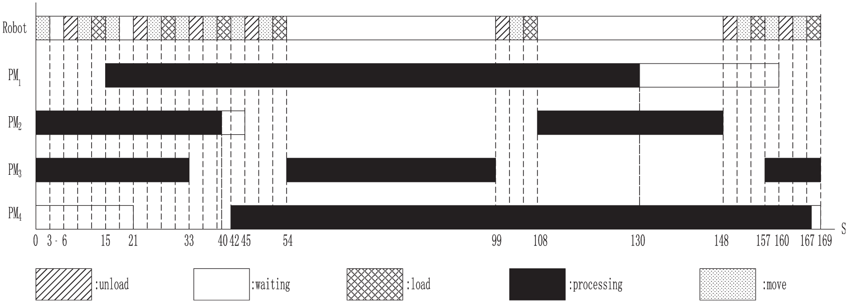
Gantt Chart for the schedule of Example 3.

Conclusion

With wafer revisiting, a single-arm cluster tool is deadlock-prone and it is very difficult to schedule such a tool to satisfy wafer residency time constraints. Thus, scheduling single-arm cluster tools with wafer revisiting and residency time constraints is very challenging. Up to now, there are studies on scheduling single-arm cluster tools with wafer revisiting or wafer residency time constraints, but not both. This work conducts a study on scheduling single-arm cluster tools with both of them for the ALD process. Based on a p-backward strategy, a PN is developed to model the process. With the model, analysis on the existence of a feasible schedule is done and schedulability conditions are established. By the proposed method, a schedule is parameterized as robot waiting time. Hence, if a feasible schedule exists, a schedule can be found very efficiently by simply setting the robot waiting time. The obtained schedule is shown to be optimal in terms of productivity.

In this article, the study is done under the assumption that wafer processing time and robot task time are deterministic. However, they may subject to random variation, which may result in infeasibility of a schedule obtained under deterministic activity time. Thus, further research is necessary to cope with this problem.