Investigation of gas–liquid two-phase flow in a three-stage rotodynamic multiphase pump via numerical simulation and visualization experiment

Abstract

To investigate the gas–liquid two-phase flow in a three-stage multiphase pump, numerical simulations and visualization experiments were performed. A mixture of air and water was selected as the medium. A three-dimensional flow field of the three-stage multiphase pump designed by authors was simulated employing the commercial computational fluid dynamics software ANSYS-CFX to solve the Navier–Stokes equations for steady flow and unsteady flow. The differential pressure of each stage and change characteristic of gas volume fraction under various inlet gas volume fraction were compared via steady simulations. The distribution characteristics of pressure and gas volume fraction in three stages were studied, and the movement of gas pockets in impellers was discovered via unsteady simulations as well. Four types of flow patterns were observed during the visualization experiments with the increasing inlet gas volume fraction. The results of the experiment reveal that the positions and characteristics of the gas pocket were similar to the results from the unsteady simulations, which verify the reliability of the simulations.

Introduction

Crude oil and natural gas are the principal sources that satisfy the energy demand of present-day industrial nations. Compared with the conventional solutions for the transportation of oil and natural gas, the multiphase pumping technique is able to pump the liquid–gas mixture with high pressure increase.^1–3 This novel solution has the following advantages:^4–7 reduction in the upfront capital outlays, reduction in the workload of management and maintenance in oil field, recovery of more oil, reduction in the risk of personal safety, and reducing environmental pollution caused by leakage during the operation of simpler facilities.

Multiphase pumps (MPPs) are mainly divided into positive displacement type and rotodynamic type. The latter type has a wide application in the subsea field due to the following advantages: smaller in size, more favorable for handling large discharge, more tolerant to sand and solids in the flow field, and more convenient utilization and maintenance. ⁸ The first reported rotodynamic MPP is called the Poseidon pump. ⁹ Through approximately decades of development, the Poseidon pump has been applied successfully in many oil fields.

Regarding theoretical research on rotodynamic MPPs, Hellmann ¹⁰ discussed forces on a single bubble. Li et al.^11–14 proposed the design method that divides all of the stages of the pump into several subsections, considering the medium in each subsection (such as three or five stages) as incompressible. Furthermore, they discussed the influence of the operating parameters on the pump’s performance and then optimized these parameters and the geometrical structure of the impeller. Yu and colleagues^15–17 conducted a hydraulic design of a rotodynamic type MPP using a combined approach of inverse design and computational fluid dynamics (CFD) analysis; in addition, the numerical simulation of gas–liquid mixture flow was also used for internal flow analysis. Zhu and colleagues^18,19 compared three different prototype pumps; they also analyzed the influence of different geometric parameters of compression cells on the hydraulic performance of the MPP. Kim et al. ²⁰ presented a design optimization to improve the hydrodynamic performance of MPPs using the design of experiment techniques.

Note that most studies on rotodynamic MPP did not discuss the effect of compressibility of the medium. In fact, the pressure will change greatly, and the gas must be compressed when the gas–liquid mixture flows through the MPP from the inlet to the outlet. As a result, it is necessary to consider the compressibility of the medium in a certain range of inlet gas volume fraction (IGVF). This article aims to study the flow field within a three-stage rotodynamic MPP. Numerical simulations of the compressible flow field will be performed to compare the pressure and the GVF in each stage at 2700 r/min while the IGVF varies from 5% to 90%.

Characteristics of rotodynamic MPP

The rotodynamic MPP is a type of multistage pump. One stage is called a compression cell, which is composed of an impeller and a diffuser, as shown in Figure 1. The suction unit, several compression cells, and the exit unit constitute the entire flow passage of an MPP. ²¹ The gas–liquid mixture gains kinetic energy while it flows through the impeller. When the mixture flows through the diffuser, its speed will decrease, and part of the kinetic energy will be converted to pressure energy. In addition, the diffuser can adjust the flow type of multiphase flow and ensure the normal operation of the next stage.

Figure 1.

Geometric model of a three-stage flow passage.

The impeller is designed to ensure the transportation of the mixture and restrain or even avoid the separation of gas and liquid. For this reason, the wrapping angle of the impeller blade is generally much larger, and the differential pressure of each stage is slightly lower.

Geometric model and mesh

The geometric model investigated in this article is composed of the extension on the front, three compression cells and the extension on the back, as described in Figure 1. The extension on the front is twice the length of the impeller, and the extension on the back is six times the length of the impeller. In addition, each impeller has 3 blades, and each diffuser has 10 blades. The three compressor cells have the same geometrical structure, which is designed based on the same operation condition.

The topological structure is used to approximate the geometric model of the flow field, and hexahedral grids are generated on it. Figure 2 describes the grid and details of the flow field. The tip clearance of an impeller is 2% of the height of the blade.

Figure 2.

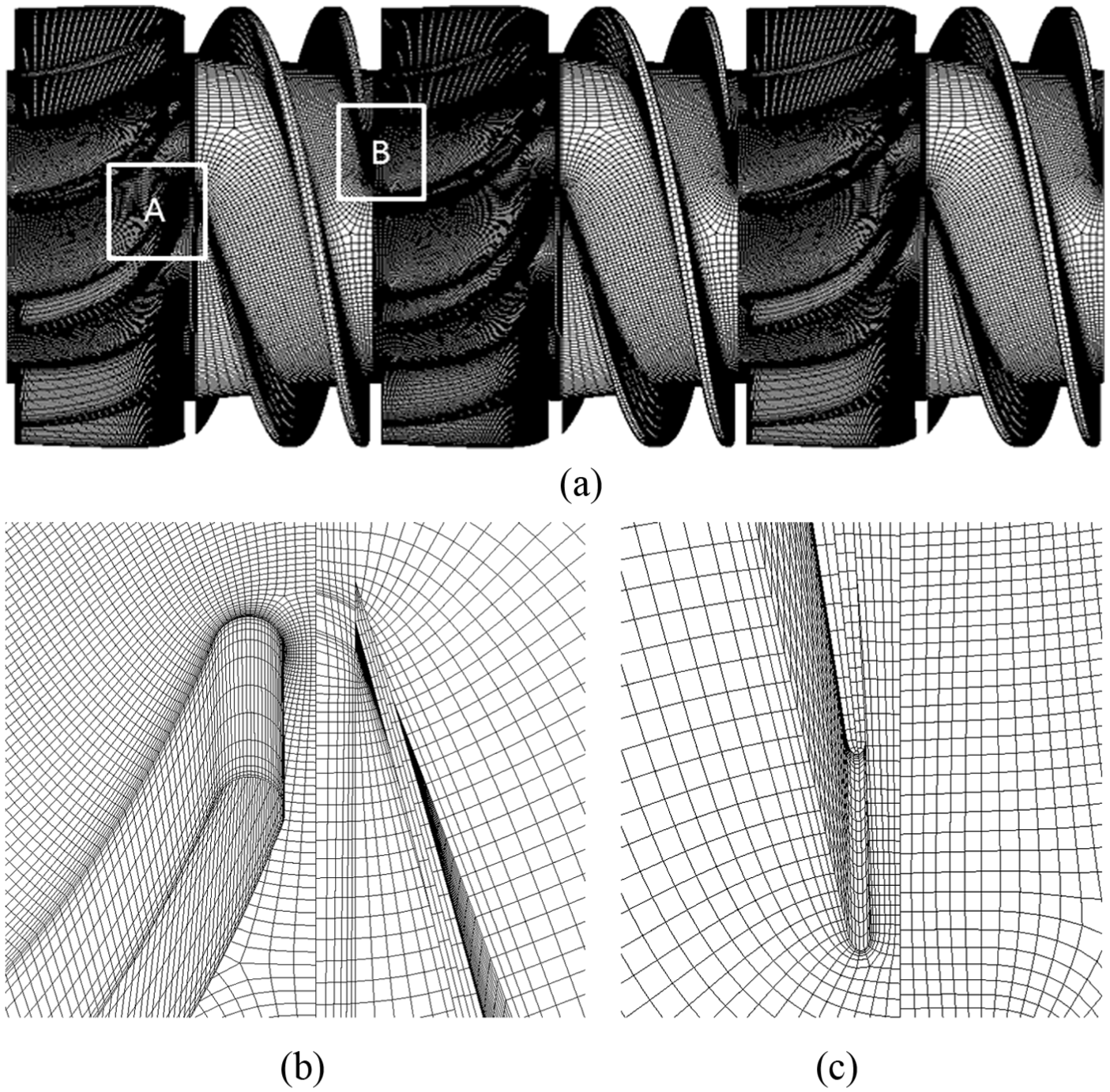
Grid and details of flow field: (a) grid on walls of impellers and diffusers, (b) grid details on region A, and (c) grid details on region B.

CFD methods

Fluid definitions

A mixture of water and ideal compressible air is chosen as the medium in this simulation. The inlet boundary condition of bubbly flow type is assumed to study the gas–liquid two-phase flow field of the pump. According to the research result in Zhang et al., ²² the bubble at the entrance of the flow field is considered as spherical, its average diameter is set, respectively, to be from 0.1 to 2.5 mm for different IGVF conditions, and the surface tension coefficient between gas and liquid is set as 0.073 N/m.

Governing equations

The Eulerian–Eulerian multiphase flow model is used in this numerical investigation. Gas and liquid both satisfy the conservations of mass and momentum. These basic equations are given as follows:

• Continuity

  $$\frac{\partial }{\partial t}({\alpha }_{\mathrm{k}}{\rho }_{\mathrm{k}})+\nabla ·\left({\alpha }_{\mathrm{k}}{\rho }_{\mathrm{k}}{\mathit{u}}_{\mathrm{k}}\right)=0$$

  (1)

• Momentum

  $$\frac{\partial }{\partial t}({\alpha }_{\mathrm{k}}{\rho }_{\mathrm{k}}{\mathit{u}}_{\mathrm{k}})+\nabla ·({\alpha }_{\mathrm{k}}{\rho }_{\mathrm{k}}{\mathit{u}}_{\mathrm{k}}\otimes {\mathit{u}}_{\mathrm{k}})=-{\alpha }_{\mathrm{k}}\nabla p_{\mathrm{k}}+\nabla ·({\alpha }_{\mathrm{k}}{\mu }_{\mathrm{k}}(\nabla {\mathit{u}}_{\mathrm{k}}+{(\nabla {\mathit{u}}_{\mathrm{k}})}^T))+{\alpha }_{\mathrm{k}}{\rho }_{\mathrm{k}}\mathit{f}+{\mathit{M}}_{\mathrm{k}}$$

  (2)

The relationship between the volume fractions of gas and liquid is shown as follows

$${\alpha }_{\mathrm{g}}+{\alpha }_l=1$$

(3)

In addition, the gas state equation of ideal compressible air is employed. For a negligible change rate of temperature, assuming that gas compression is isothermal, the equation of the gas state is

$$p_0{Q}_{\mathrm{g}0}=p{Q}_{\mathrm{g}}=\mathrm{const}$$

(4)

Interphase forces

The forces acting on two phases are usually divided into three parts: interphase drag force ${\mathit{M}}_{\mathrm{k}}^{\mathrm{D}}$ , lift force ${\mathit{M}}_{\mathrm{k}}^{\mathrm{L}}$ , and virtual mass force ${\mathit{M}}_{\mathrm{k}}^{\mathrm{A}}$ ; thus, the interphase force is ${\mathit{M}}_k={\mathit{M}}_{\mathrm{k}}^{\mathrm{D}}+{\mathit{M}}_{\mathrm{k}}^{\mathrm{L}}+{\mathit{M}}_{\mathrm{k}}^{\mathrm{A}}$

$${\mathit{M}}_{\mathrm{k}}^{\mathrm{D}}=\frac{3}{8}\frac{C_{\mathrm{D}}}{r_{\mathrm{g}}}{\rho }_l({\mathit{u}}_{\mathrm{l}}-{\mathit{u}}_{\mathrm{g}})|{\mathit{u}}_{\mathrm{l}}-{\mathit{u}}_{\mathrm{g}}|$$

(5)

$$C_{\mathrm{D}}=\{\begin{array}{cc}\hfill 24(1+0.15{\mathrm{Re}}^{0.687})/\mathrm{Re}\hfill & \hfill \mathrm{Re}\le 1000\hfill \\ \multicolumn{1}{c}{0.44}& \hfill \mathrm{Re}>1000\hfill \end{array}$$

(6)

$\mathrm{Re}$ is calculated as follows

$$\mathrm{Re}={\rho }_l\frac{|{\mathit{u}}_l-{\mathit{u}}_g|}{{\mu }_l}{d}_{\mathrm{g}}$$

(7)

$${\mathit{M}}_{\mathrm{k}}^{\mathrm{L}}=C_L{\rho }_l{\alpha }_g{\mathit{u}}_R\times (\nabla \times {\mathit{u}}_l)$$

(8)

where ${\mathit{u}}_{\mathrm{R}}={\mathit{u}}_{\mathrm{g}}-{\mathit{u}}_l$ , $C_{\mathrm{L}}=0.5[1.0-2.78〈0.2,{\alpha }_{\mathrm{g}}〉]$ , and $〈a,b〉$ mean selecting the minimum value between a and b

$${\mathit{M}}_{\mathrm{k}}^{\mathrm{A}}={\rho }_l{C}_{\mathrm{A}}{\alpha }_{\mathrm{g}}{\mathit{a}}_{\mathrm{A}}$$

(9)

This article assumes that a bubble is spherical, so $C_{\mathrm{A}}$ is set to 0.5, and ${\mathit{a}}_{\mathrm{A}}$ is expressed as

$${\mathit{a}}_A=\frac{\partial {\mathit{u}}_{\mathrm{R}}}{\partial t}+{\mathit{u}}_{\mathrm{g}}·\nabla {\mathit{u}}_{\mathrm{g}}-{\mathit{u}}_l·\nabla {\mathit{u}}_l$$

(10)

Method of solution and boundary conditions

As inhomogeneous multiphase models are used in this simulation, different turbulence models are adopted for liquid and gas. In addition, the Semi-Implicit Method for Pressure-Linked Equations (SIMPLE) method is set to solve for the pressure and velocity. The governing equations are calculated using the finite volume method, and the method of pressure interpolation is PREssure STaggering Option (PRESTO). In the process of simulation, the following assumptions are used: (1) the two-phase mixture is homogeneous at the inlet surface of flow field; (2) the main phase is the incompressible continuous liquid, and the gas phase mixed with the liquid behaves as an ideal compressible gas; (3) there is no mass transfer between the two phases; and (4) there is no cavitation phenomenon within the MPP. The detailed information regarding the method of solution and the boundary conditions are presented in Table 1.

Table 1.

Basic setting for the solution and the boundary conditions.

Component	Feature	Details
Calculation method	Analysis type	Steady and unsteady
	Medium	Mixture of water and ideal compressible air
Turbulence models	Water	k-ω SST
	Air ideal gas	Dispersed-phase zero equation model
Solve control	Discretization	First-order upwind scheme for the GVF term Second-order upwind scheme for the other terms
	Maximum residual	10−6 for mass, momentum, and energy 10−3 for the mass balance and torque of each stage
Boundary conditions	Inlet	Mass flow (kg/s) and GVF
	Outlet	Average pressure (MPa)
	Domain interfaces	Frozen rotor for steady simulation
		Transient frozen rotor for unsteady simulation
	Wall	No slip, isothermal (25°C)
Transient time option	Time step	1.85e−4 s

GVF: gas volume fraction; SST: shear stress transport.

Mesh independence

To shorten the time and improve the accuracy of the computation, the optimum number of grid cells in the simulation was investigated. Considering the great number of grid points in the three-stage pump, a large amount of Central Processing Units (CPUs) power and time are required to finish the simulation. In addition, the mesh of the impeller is the key factor for the accuracy of this simulation. In this article, a new geometrical model with the same impeller and without a diffuser (shown in Figure 3) is created. Given that the hydraulic performance of the three-stage pump mainly depends on the impellers, the mesh of an impeller is used to verify the mesh independence. In addition, the differential pressure between the inlet and the outlet of the impeller and the hydraulic efficiency of the impeller are used to evaluate the eight grids (shown in Table 2) and determine the influence of the mesh size on the solution.

Figure 3.

Geometric model used to verify the mesh independence.

Table 2.

Evaluated grid cells.

Characteristics	Number of cells	Differential pressure (MPa)	Hydraulic efficiency (%)
Grid A	160,518	0.07485	52.907
Grid B	193,842	0.07409	53.946
Grid C	227,166	0.07376	54.315
Grid D	310,476	0.07417	54.434
Grid E	410,448	0.07425	54.519
Grid F	493,758	0.0743	54.520
Grid G	577,068	0.07432	54.520
Grid H	743,688	0.07432	54.520

From Table 2, the differential pressure and hydraulic efficiency are found to reach an asymptotic value as the number of cells increases. According to this table, when the number of cells is greater than 410,448, the change in the differential pressure is less than 0.8 × 10⁻³ MPa, and the hydraulic efficiency is less than 0.2%. Thus, Grid E (410,448 cells) is considered to be sufficiently reliable to ensure mesh independence. Table 3 presents the final grid number of every component of the three-stage MPP used in this article. According to Table 3, the total mesh number can be calculated is 6,604,406 for the three-stage flow field.

Table 3.

Grid cells in different parts.

Different parts of the model	Number of cells
Extension on the front	147,670
Each impeller	410,448
Each diffuser	1,410,464
Extension on the back	994,000

Results of simulations

ANSYS-CFX software is used to simulate the steady and unsteady flows in the three-stage rotodynamic MPP. The differential pressure and GVF in three compressor cells are compared according to the results of steady simulation. An unsteady simulation is performed to investigate the flow characteristics of air, which has a very important significance on the hydraulic performance of the pump.

Steady flow

Some flow parameters, such as total flow rate, rotational speed, and IGVF, influence the hydraulic performance of the pump. Note that IGVF is the most influential parameter for an MPP. In the process of steady simulation, IGVF changes from 5% to 90%, while the rotational speed and total flow rate are kept unchanged as 2700 r/min and 35 m³/h.

Differential pressure of each compression cell

The average static pressure along the axial direction from the inlet to the outlet under 30% IGVF condition is described in Figure 4. It can be seen that the differential pressure of each stage increases successively from the first stage to the third one. This phenomenon occurs mainly due to the compressibility of gas, which also leads to the decrease in the GVF and the total volume flow of mixture. The pressure increases slightly at each diffuser because it converts part of the kinetic energy into pressure energy. The average pressure declines slightly at the interfaces between rotors and stators, which results from the effect of their interaction.

Figure 4.

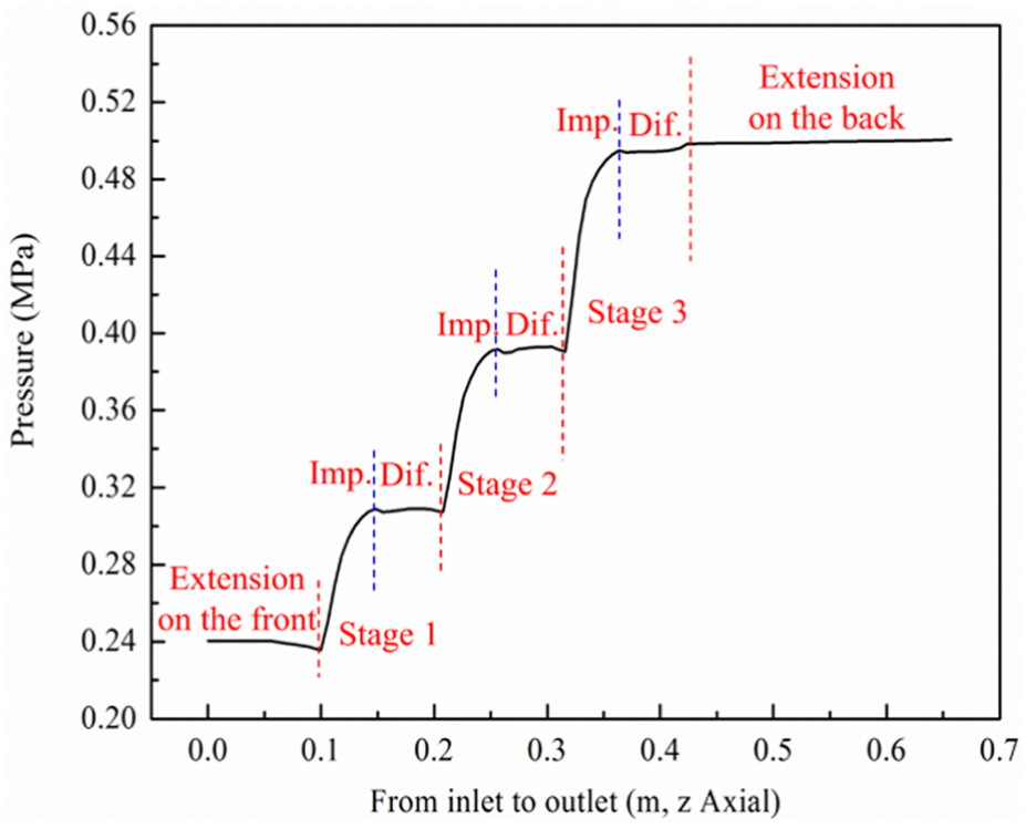
Change in the average static pressure along the axial direction.

Figure 5 shows the differential pressure of the three stages with the increasing IGVF when the total volume flow and rotational speed remain unchanged. It can be seen that the differential pressure of three stages decreases slowly with the increasing IGVF. At the same IGVF condition, the differential pressure of single stage increases gradually from the first stage to the third one due to the compressibility of air, which results in the decrease in total flow rate.

Figure 5.

Differential pressure versus IGVF of the three stages.

Average GVF change rate of three stages

With the variation of IGVF from 5% to 90%, the average GVF distribution in different sections from inlet to outlet is described in Figure 6. We can see that the average GVFs in the researched sections decrease as a whole from inlet to outlet of the whole flow field. It results from the combined action of pressure boost and compressibility of mixture. However, the extent and rate of average GVF decreasing under various IGVF conditions are not the same. The change is relatively small under 5% and 90% IGVF conditions. Consequently, the compressibility of mixture will be not obvious if the IGVF is too high or too low.

Figure 6.

Average GVF distributions in different sections with various IGVF.

Unsteady simulation

To investigate the flow of gas–liquid two-phase within the three-stage rotodynamic MPP dynamically, unsteady simulations are conducted based on the steady simulation results with the above conditions. In the process of the unsteady simulation, the time step is set as 1.85e⁻⁴ s based on the typical cell size and the characteristic flow velocity. According to the speed of the pump (2700 r/min), the impeller rotates 2.997° in one time step. The condition of 30% IGVF is taken as an example to analyze the unsteady flow field of the pump.

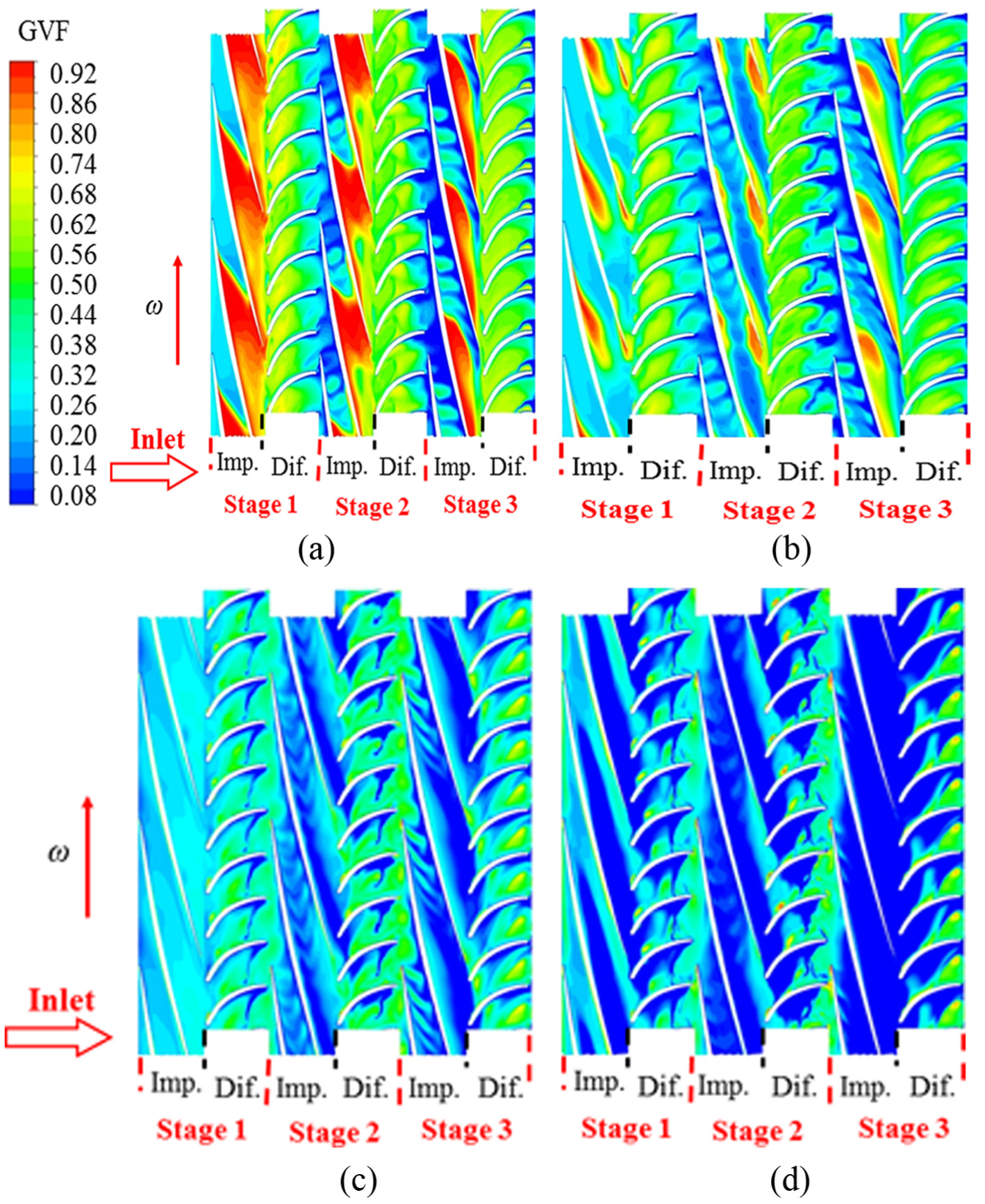
Figure 7 shows the average GVF in the meridional plane of the three compressor cells obtained from the unsteady simulation. The GVF is higher near the hub, while it is lower near the shroud as shown in Figure 7. The areas of higher GVFs decrease gradually from the first to the third stage. This behavior occurs because the fluid in the rotational impellers is influenced by the centrifugal force, which causes water to move toward the shroud of the impeller and air to gather near the hub. The diffusers are stationary parts that have the ability to adjust the fluid field and eliminate the centrifugal force. Thus, the areas of higher GVF near the hub and the areas of lower GVF near the shroud disappear gradually in diffusers. However, there are large areas of higher GVF near the hub at the inlet of each diffuser, where a vortex is observed according to the velocity vectors, as shown in Figure 8. A small area of higher GVF is also found near span 0.8 in the interfaces of the diffuser and the impeller. The effect of rotor–stator interaction is the main reason for this small area. This small area of higher GVF can also be explained by the velocity vectors shown in Figure 8. Near span 0.8, an obvious vortex exists, which causes the higher GVF to occur there. Compared with the first and second stages, no obvious higher GVF is found at the outlet of the diffuser of the third stage. A long extension behind the third stage ensures the fluid as the outlet of diffuser is not affected by the effect of rotor–stator interaction, so the velocity vectors are more regular, as shown in Figure 9.

Figure 7.

Average GVF in the meridional plan of the three stages.

Figure 8.

Velocity vector in the second diffuser.

Figure 9.

Velocity vector in the third diffuser.

Generation of the gas pocket

Figure 10 shows the GVF distribution on the cascade planes of different blade spans. From the distribution characteristic of the GVF obtained from the unsteady simulation, we find that the gas flowing from the inlet to the outlet of impellers is not continuous but is a series of spaced air masses gradually moving toward the outlet of the impeller.

Figure 10.

GVF distributions on the cascade planes of different spans: (a) span 0.1, (b) span 0.3, (c) span 0.5, and (d) span 0.9.

From the impeller span range of 0.1 to 0.9, the area of higher GVF decreased gradually, especially near the shroud (span 0.9) of the impeller, with the higher GVF only appearing in the diffusers. All of these results indicate that the air mainly gathers near the hub. At impeller span 0.1, the distributions of higher GVF regions in three impellers are different. In the impeller of the first stage, the area of higher GVF is the largest and even extends from the pressure surface to the suction surface of blades. In the impeller of the second stage, the area of higher GVF decreases but still stretches from the pressure surface to the suction surface of blades. In addition, affected by the interaction between rotor and stator, the distribution of the GVF is more disordered than in the first stage. In the impeller of the third stage, the higher GVF region is close to the pressure surface but no longer extends to the suction side. At impeller span 0.3, the area of higher GVF can still be observed in the impeller passage. Similar to the impeller span 0.1, there are areas of higher GVF on both suction and pressure surfaces, while the area decreases obviously, and the regions of higher GVF are separated from the pressure surface to the suction surface. At impeller spans 0.5 and 0.9, the areas of higher GVF almost cannot be observed. On the contrary, there are large areas of the lower GVF region. The lower GVF area increases gradually from the first impeller to the third impeller.

The growth and collapse of the gas pocket

The second- and third-stage impellers are all affected by the interaction of both upstream and downstream diffusers. Thus, they have similar change rules of the GVF. In addition, the movement rules of air in the two impellers can represent the normal states in a multistage MPP. Here, part of the cascade plane includes the second-stage diffuser, and the whole third stage is selected as an example for the further analysis described below.

Figure 11 shows the change rules of GVF with time at the selected cascade plane. With the continuous rotation of the impeller, the leading edges of the impeller constantly cut the mixture out of the front diffuser. As shown in Figure 11, there is a region of lower GVF after the trailing edges of the diffuser. As shown in the dotted rectangle in Figure 11, at time step t, the leading edge of the impeller moves to the trailing edge of the diffuser, and the mass of fluid with lower GVF enters the passage of the impeller along with the leading edge. At time step t + 5Δt, a small gas mass appears at the leading edge of the impeller, while it passes a passage between two blades of the front diffuser. With the impeller rotating, some gas masses form one by one. Ultimately, a series of discrete gas masses move downstream along the passages of the impeller and enter the large gas pocket. At the same time, some gas flows out from the gas pocket to the downstream diffuser. Thus, the area of the gas pocket reached a saturation situation.

Figure 11.

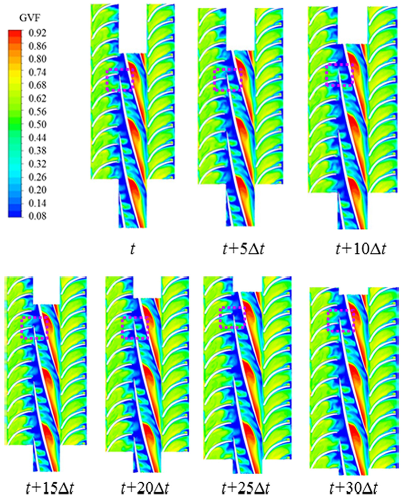
GVF distributions on the selected cascade plane at different time steps.

Figure 12 shows the distribution of the pressure changes with time at the same position as in Figure 11. However, the time steps are selected as a blade of the impeller rotating passes a passage of the diffuser. The pressure is found to change periodically due to the interaction between one impeller and two diffusers.

Figure 12.

Pressure distributions on the cascade plane at different time steps.

Initially, the change of the flow field in the diffusers and the impeller can be observed when the leading edges of the impeller pass the trailing edges of the front diffuser. Here, consider the two flow passages of the diffuser as the focus of the study. These flow passages are labeled “a” and “b.” At time t, one blade leading edge of the impeller moves to passage “b.” The pressure in passage “b” is found to be higher than the pressure in passage “a.” In particular, there is an obvious higher pressure region on the pressure surface at the head of the impeller blade. At time t + 2Δt, the pressure decreases obviously in passage “b” compared with the pressure at time t, while the pressure increases in passage “a.” From time t + 4Δt to time t + 8Δt, the pressure increases obviously in passage “a,” while it decreases gradually in passage “b” as the leading edge of the impeller blade gradually approaches the trailing edge of the diffuser blade. At time t + 12Δt, the leading edge of the impeller blade passed the trailing edge of the diffuser blade and entered passage “b.” At the same time, the pressure reaches its maximum in passage “a,” while it decreases to its minimum in passage “b.” Opposite to the results at time t, passage “a” becomes the higher pressure region and passage “b” becomes the lower pressure region at time t + 12Δt. It can be deduced that the pressure distribution in diffusers will be periodically affected by the rotational impeller.

Furthermore, the pressure change associated with the interaction between the impeller and the diffuser can be analyzed while the trailing edge of the impeller blade passes the leading edge of the downstream diffuser blade. As shown in the position of the dotted lines in Figure 12, from time t to time t + 4Δt, the trailing edge of the impeller blade gradually approaches the leading edge of the downstream diffuser blade. Meanwhile, the pressure on the interface increases gradually. The area of high pressure increases obviously at time t + 6Δt. From time t + 6Δt to time t + 12Δt, the trailing edge of the impeller blade detaches from the leading edge of the downstream diffuser blade, and the area of high pressure decreases gradually. From time t to time t + 12Δt, the pressure of each passage in the downstream diffuser also periodically changes.

Visualization experiment

Test bench

The test bench for this research in the laboratory consists of an open-type gas circuit and a closed-cycle water-flow loop. The test bench includes an MPP, a buffer tank, a transducer, a water tank, a line pump, an electric motor, a high-speed camera, some pressure transmitters and flow meters, and so on. The sketch of the experiment rig is shown in Figure 13. The testing media is the mixture of air and water. Under the two-phase conditions, before being pumped by the MPP, the mixture is transported into the buffer tank to first be mixed uniformly. Ultimately, the mixture is carried into the water tank from the outlet of the MPP. The tank is large enough to ensure that the air is released into the environment and the water flows cyclically.

Figure 13.

Test bench of the three-stage multiphase pump.

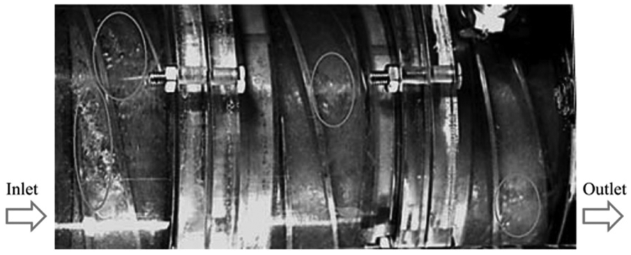
The shell of the pump is produced with organic glass for the observation of flow field. The type of high-speed camera used is NorPix FR-625, which has a maximum resolution of 1280 × 1024 and a maximum frame rate of 5000 fps.

The automatic data acquisition system and automatic control system of the valves are used for collecting the data. Several pressure transmitters and two flow regulation valves are installed. The data acquisition board with functions of A/D and D/A is used for data acquisition and flow control of both water and air. This process is operated automatically by acquisition and control software. Table 4 presents the details of the various measuring equipment (for determining Q, P, T, etc.) and their uncertainty.

Table 4.

Details of the various pieces of measuring equipment.

Parameters	Measuring equipment	Range of measurement	Uncertainty (%)
Q g	LWQ-50 turbine flow meter	5–100 m3/h	1.5
v l	LDBE-80 electromagnetic flow meter	0.3–15 m/s	0.5
P	1151 series of pressure transmitter	0–1.6 MPa	0.1
T	Torque meter	0–500 N	0.2

In addition, the GVF in different points can be calculated. The flow rate and pressure can be measured before the water and air enter the mixing device. A capacitance differential pressure transmitter is added in the inlet of MPP. The IGVF can be obtained based on the energy conservation equation.

Analysis of the results

Analysis of the flow patterns in the impellers

This experiment primarily involves the study of the flow pattern in impellers with the increasing IGVF under the same rotational speed. A high-speed photography system is used to observe the two-phase flow pattern and the movement of air within the MPP. As shown in Figure 14, the experimental results show that the flow patterns in the impellers of the MPP can be classified into four categories with the increasing IGVF: isolated bubble flow, bubbly flow, gas pocket flow, and segregated gas flow. In addition, the independently designed buffer tank ensures that the flow pattern at the inlet of pump is bubbly flow, which verifies the rationality assumption for the inlet boundary condition in the numerical simulations.

Figure 14.

Flow patterns in the first impeller: (a) isolated bubble flow, (b) bubbly flow, (c) gas pocket flow, and (d) segregated gas flow.

Bubbles gather more intensively when the flow pattern is in the form of gas pocket flow. Massive bubbles in the passages of impellers are gathered into gas pockets that are located in the pressure surface near the outlet of the impeller. The existence of gas pockets makes the flow area of the passages smaller, which lead to the increase in relative velocity of the fluid. In this case, the flow loss will increase and the hydraulic performance will decrease sharply. The pressure, flow rate, and shaft power at the inlet and outlet will fluctuate obviously and the vibration and noise also increase. In the flow pattern of the segregated gas flow, the passage can be divided into two regions: a white region (which consists mainly of air) and a transparent region (which consists mainly of water). Generally, the white region is close to the hub, while the transparent region is near the shroud. Gas pockets still exist, but they are covered by the white region and cannot be observed clearly. The detailed analysis from the visualization experiment is presented in Zhang et al. ²³

Position analysis of gas pockets

When the flow pattern is gas pocket flow, gas pockets can be clearly observed from both the simulation and the experiment, as shown in Figures 15 and 16. The threshold GVF value in Figure 15 is 0.85. The position analysis of the gas pockets is as follows: from the simulation results shown in Figure 15, the areas of gas pockets are found to decrease from the first stage to the third one. These areas are mainly located near the hub of the impellers. In the process of experiment, gas pockets first appeared in the first stage, and there is no large isolated bubble around them, which means that isolated bubbles gathered in the gas pockets. The gas pockets in the second stage, for both the simulation and experimental results, remain located near the hub and close to the pressure surface of blades in the impeller, as in the first stage, but they are closer to the outlet of the impeller along the axial direction. Due to the compressibility of air, the size of the gas pockets in the second stage is smaller than the size in the first stage. In contrast to the second stage, the locations of the gas pockets in the third impeller are closer to the outlet of impeller. In addition, the areas of the gas pockets in the third impeller are the minimum among the three impellers.

Figure 15.

Gas pockets obtained from the simulation.

Figure 16.

Gas pockets obtained from the visualization experiment.

Conclusion

The gas–liquid two-phase flow in a three-stage MPP was investigated via numerical simulation and visualization experiment with the media of mixture of water and air. The visualization experiment presented four main gas–liquid two-phase flow patterns. The characteristics of the gas pockets showed in the experiment were similar to that obtained from the unsteady simulation.

Both numerical simulation and visualization experiment show that the compressibility of gas and centrifugal force affected, obviously, the flow field and performances of MPP. The difference of centrifugal forces acted on liquid and gas results the gas to gather near the hubs of impellers. The compressibility of gas resulted in the difference of GVF distribution and differential pressure of each stage. So, the impellers of MPP must be designed stage by stage based on the compressibility of the gas.

Furthermore, the effect of rotor–stator interaction acted an obvious rule on the generation of gas pockets in impellers. Rotor–stator interaction also causes many obvious vortices in every passage of the diffusers. Air gathering and retention occur in diffusers. Air mainly gathers in the center of the vorticity. The generation and development of gas pockets with time in impellers can be explained for the combined actions of centrifugal force, rotor–stator interaction, vorticity, and the non-homogeneous pressure distribution.