Sage Journals: Discover world-class research

Abstract

To improve the condition of air and eliminate exhaust gas pollution, this article proposes a compressed air power system. Instead of an internal combustion engine, the automobile is equipped with a compressed air engine, which transforms the energy of compressed air into mechanical motion energy. A prototype was built, and the compressed air engine was tested on an experimental platform. The output torque and energy efficiency were obtained from experimental results. When the supply pressure was set at 2 MPa and the speed was 420 r min⁻¹, the output torque, the output power, and the energy efficiency were 56 N m, 1.93 kW, and 25%, respectively. To improve the efficiency of the system, a fuzzy logic speed control strategy is proposed and simulated. The experimental study verified that the theoretical evaluation of the system was reasonable, and this research can be referred to as the design and control of air-powered vehicles.

Keywords

Compressed air power automobile experimental platform speed control

Introduction

Air pollution, especially by atmospheric fine particles, has been a severe problem for many years. The burning of fossil fuels through internal combustion engines in transportation vehicles has been a major source of this kind of air pollution.^1,2 According to relevant research reports, atmospheric fine particles (particulate matter 2.5 (PM2.5)) produced by automobiles are responsible for >30% of the air pollutants in Beijing.³ The problem will continue to worsen as the number of automobiles increases. This environmental threat has made it imperative to develop a viable alternative to fossil fuels for transportation vehicles. This work presents an engine using compressed air as a possible solution.^4,5

Instead of an internal combustion engine, the automobile is equipped with a compressed air engine (CAE), which transforms the energy of compressed air into mechanical motion energy. Compared with other eco-automobiles, this automobile promises high efficiency, high maturity, and completely zero emissions. Therefore, this prospect has drawn the attention of scholars.⁶

David Huang and Tzeng⁷ and David Huang et al.⁸ proposed an innovative concept—a hybrid pneumatic power system (HPPS) ensures that the internal combustion operates optimally and recycles the exhaust energy, thereby increasing the vehicle’s efficiency. Shaw et al. analyzed a compressed air–pressurized hydraulic oil hybrid pneumatic system. In their system, the energy was transformed to mechanical energy by a hydraulic motor to improve the efficiency of using air power.⁹ It is obvious that compressed air provides auxiliary energy for most hydraulic systems. The blending with bio-diesel¹⁰ augments the naturally available fossil fuel, but this fuel still remains a limited resource and does not meet the zero pollution vehicle (ZPV) requirements. With the development of the technology of compressed air energy storage, the utilization of compressed air in transport vehicles and other utilities is an attractive option, especially in view of its potential as a ZPV alternative.

There are many types of CAEs that can be applied to a transportation vehicle. Various types, such as vane, rotary piston, and piston, are being constantly evaluated across the world. Singh and Singh designed a vane-type air turbine. To maximize shaft work, different aspects of improving efficiency were proposed.¹¹ Singh and Singh⁴ also optimized the multi-vane air engine injection method and the vane angles to improve performance. Shen and Hwang presented an idea of using compressed air as the power source for motorcycles. A fuzzy logic speed controller was applied in a prototype.¹² Engineair is a company focused on the development of air motor technology based on a unique rotary piston concept. Commercial products had already been designed.¹³ Compared with other air-powered engines, the piston-type CAE promises high compressed air pressure, high efficiency, and high maturity and, therefore, draws the attention of scholars. Huang et al.¹⁴ modified a CAE with a 100-cm³ internal combustion engine and investigated its performance experimentally. Motor Development International (MDI) holds international patents for piston-type CAEs.¹⁵ Chen et al.¹⁶ proposed a newly electro-pneumatic valve for the compressed air-powered engine. Although many have proposed that the output power and efficiency are affected by speed during operation, relatively few studies have reported speed characteristics and a control strategy for piston-type CAEs while working. This study focuses on the speed characteristics and speed control during operation.

This article presents a prototype using piston-type CAEs with the benefit of eliminating the release of pollutant exhaust gases to the atmosphere. The efficiency of this CAE is analyzed through experiment data. Reasonable speed can be obtained by efficiency analysis. A fuzzy logic speed controller is also developed to maintain reasonable speed. The remaining sections are organized as follows: an introduction to CAEs is described in section “Introduction of the air-powered vehicle system,” a theoretical analysis is carried out in section “Theoretical analysis,” experimental results are shown and analyzed in section “Simulation study and experimental verification,” a fuzzy logic speed controller is presented in section “Fuzzy control design,” and the conclusions are stated in section “Conclusion.”

Introduction of the air-powered vehicle system

The structure of a piston-type CAE is shown in Figure 1, and the main parts are labeled. To obtain a fast response in terms of valve moment, the input flow of the CAE is controlled by a cam.

Figure 1.

Piston-type CAE.

In a suction power stroke, the compressed air flows into the cylinder through an intake valve and the piston are driven downward. The linear movement of the piston is converted to rotary motion by a crank-connecting rod mechanism. The intake angle and phases are decided by the cam profile. When the intake valve closes after a specific crank angle, the compressed air inside the cylinder expands and pushes the piston down. This process causes the exhaust valve to close.

When the piston is near the bottom dead center (BDC), the exhaust valve opens so that the air, with residual pressure, discharges under the impetus of the piston. The piston is then driven by the flywheel energy and finally arrives at the top dead center (TDC).

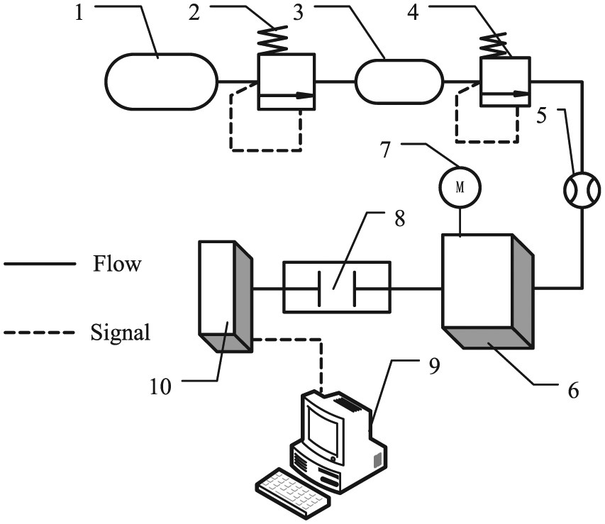
The air-powered vehicle (APV) system, whose schematic diagram is shown in Figure 2, consists of a CAE, a carbon-fiber tank, an electronic proportional directional control valve (SMC ITV1050), an air control valve (TESCOM), two regulators (TESCOM), a buffer tank, a pressure sensor, a speed sensor, an accelerator pedal, and an electrical control unit. The pressure entering into the CAE will be determined by the air control valve position, which is controlled by the ITV1050 exhaust pressure. The ITV1050 exhaust pressure is determined by an externally applied electric current, denoted by I. When I is equal to 4 mA, the valve closes. When I is equal to 20 mA, the valve is fully open. The electric current is controlled by an electrical control unit. The major elements of the APV system and their functions are listed in Table 1.

Figure 2.

Schematic diagram of the power system of the APV.

Table 1.

APV equipment.

Elements	Function
1. High-pressure gas tank	Store and provide high-pressure gas
2. High-pressure regulator	Modulate pressure to meet buffer tank
3. Buffer tank	Stabilize pressure fluctuation and absorb energy from surroundings
4. Pressure sensor	Obtain the pressure of supply gas
5. Regulator	Regulate gas pressure to meet ITV1050
6. Proportional directional control valve	Modulate the pressure of entering air, which controls the elements
7. Electrical control unit	Obtain sensor and pedal signals, output the analog signal to the electronic control valve
8. Accelerator pedal	Export user command
9. Air control valve	Modulate the pressure of entering air
10. Speed sensor	Measures the speed of the CAE
11. CAE	Transforms the energy of the compressed air into mechanical motion energy

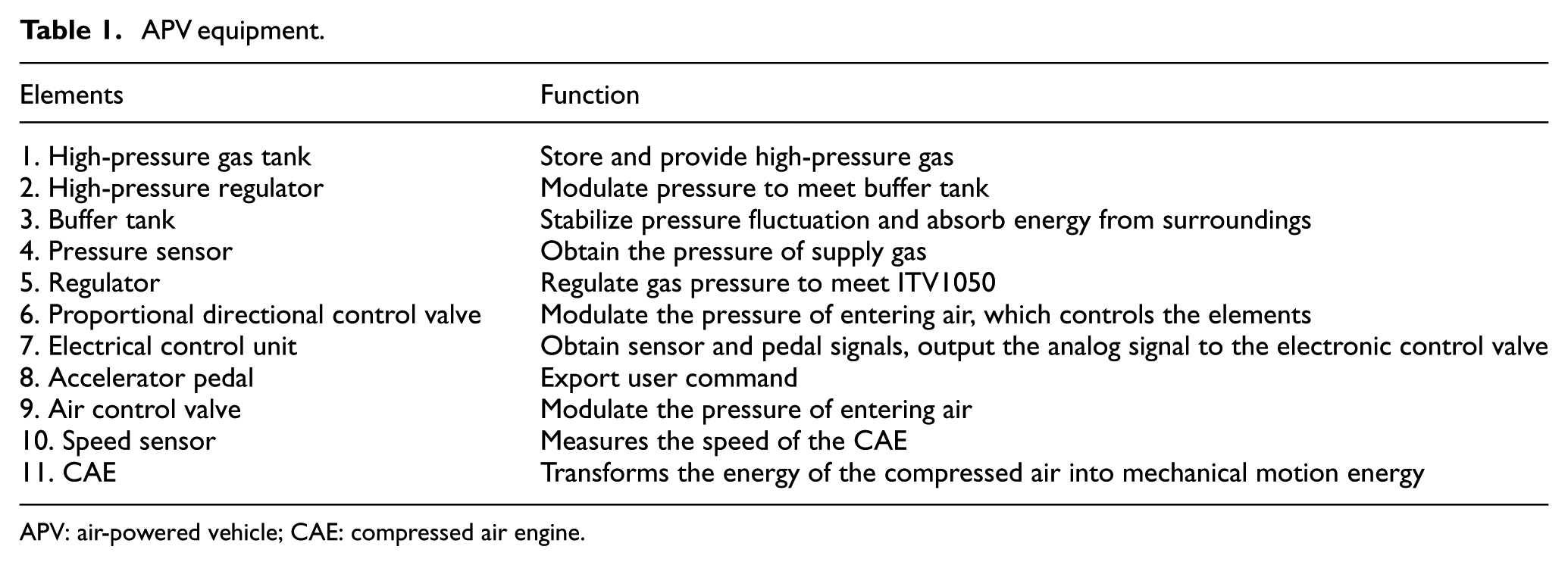
APV: air-powered vehicle; CAE: compressed air engine.

Theoretical analysis

System simplification

To facilitate this research, the following necessary assumptions are made:

Each point in the interconnecting conduit has some pressure. This requires ignoring the pressure loss along the pipe.

There is no leakage during the working cycle.

The volume of the pipe is neglected.

The regulator and valve are considered a throttle orifice.

The APV system can be simplified using these assumptions, and a schematic diagram is shown in Figure 3.

Figure 3.

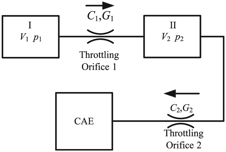
Simplified APV system.

The arrow indicates the direction of flow. Volume I is a high-pressure tank chamber. Volume II is a buffer tank chamber. Throttling orifice 1 represents the high-pressure regulator. Throttling orifice 2 represents elements 5, 6, and 9, which are shown in Figure 2.

Mathematical modeling of the APV system

The APV system includes three major parts: a gas tank, a pressure regulator, and a CAE. Therefore, the system model required by the quantitative simulation includes all three major parts and is described in the following.

Gas tank

State equation

The purpose of the gas tank is to provide energy for running the CAE. The air pressure in the tank was set at 30 MPa to obtain a high power density and enough energy. According to the literature,¹⁷ the gas can be approximated as an ideal gas if the pressure p < 0.5p_c or the temperature T > 5T_c. From the literature,¹⁸ the critical pressure (p_c) and temperature (T_c) of air are 3.77 MPa and 132.42 K, respectively. Many equations such as the Soave–Redlich–Kwong(S-R-K)¹⁹ and the Peng–Robinson (P-R)²⁰ have been proposed about real gas. Here, the real gas van der Waals state equation²¹ was applied, as shown in equation (1)

(p_{i} + \frac{a}{v_{i}^{2}}) (v_{i} - b) = R T_{i}

(1)

v_{i} = V_{i} \frac{M}{m_{i}}

(2)

where p_i is the pressure of the air in the gas tank (Pa), V_i is the volume of the air in the gas tank (m³), v_i is the volume of the container occupied by each particle, m_i is the mass of the air in the gas tank (kg), a is a measure of the attraction between the particles (Pa m⁶ mol⁻²), b is a correction term based on the molecular volume(m³ mol⁻¹) of the gas, M is molar mass (g mol⁻¹), and R is the ideal gas constant (R = 8.3143 J mol⁻¹ K⁻¹). For air, the values of a, b, and M are 0.1358, 0.0000367, and 28.97, respectively. The subscript i represents 1 and 2, as labeled in Figure 2.

Based on equations (1) and (2), the pressure differential equation is given as

\begin{matrix} (\frac{V_{i}}{m_{i}} - \frac{b}{M_{i}}) \frac{d p_{i}}{dt} + (\frac{p_{i}}{m_{i}} - \frac{a m_{i}}{V_{i}^{2} M} + \frac{2 {abm}_{i}^{2}}{V_{i}^{3} M^{3}}) \frac{d V_{i}}{dt} \\ + (\frac{a}{V_{i} M^{2}} - \frac{p_{i} V_{i}}{m_{i}^{2}} - \frac{2 ab m_{i}}{V_{i}^{2} M^{3}}) G_{i} = R \frac{d T_{i}}{dt} \end{matrix}

(3)

Because the volume is constant, dV_i/dt is equal to 0. Therefore, equation (3) can be simplified to equation (4)

(\frac{V_{i}}{m_{i}} - \frac{b}{M_{i}}) \frac{d p_{i}}{dt} + (\frac{a}{V_{i} M^{2}} - \frac{p_{i} V_{i}}{m_{i}^{2}} - \frac{2 ab m_{i}}{V_{i}^{2} M^{3}}) G_{i} = R \frac{d T_{i}}{dt}

(4)

Energy equation

The energy equation²² can be given in the form of the temperature differential equation

\frac{dT}{dt} = \frac{1}{m_{i} C_{v}} [c_{hi} A_{hi} (T_{a} - T) + h_{in} G_{in} + h_{out} G_{out} - uG]

(5)

where G_in = dm_in/dt; G_out = dm_out/dt; G = dm_i/dt; C_v is the constant volume specific heat (J kg⁻¹ K⁻¹); C_hi is the heat transfer coefficient; A_hi is the total heat transfer area (m²); T_a is the temperature of the internal walls (K); h_in and h_out are the specific enthalpies of the air flow into and out from the cylinder, respectively; m_in and m_out are the masses of the air flow in and out, respectively; and u is the specific internal energy.

Pressure regulator

Continuity equation

According to the literature,²³ the pressure regulator can be considered to have an air resistance factor. The air flow of the orifice throttle can be calculated as follows

G_{i} = {\begin{matrix} ρ_{0} C_{i} p_{u} \sqrt{\frac{293}{T_{u}}} & \frac{p_{d}}{p_{u}} \leq 0.5 \\ ρ_{0} C_{i} p_{u} \sqrt{\frac{293}{T_{u}}} \cdot \sqrt{1 - {(\frac{\frac{p_{d}}{p_{u}} - 0.5}{1 - 0.5})}^{2}} & \frac{p_{d}}{p_{u}} > 0.5 \end{matrix}

(6)

where C_i is the sonic conductance (dm³ s⁻¹ bar⁻¹), ρ₀ is the gas density under standard conditions (kg m⁻³), p_u is the upstream pressure (Pa), and p_d is the downstream pressure (Pa). In case of the air, the value of ρ₀ is 1.185, and subscript i values of 1 and 2 represent the intake and exhaust ports, respectively.

Joule–Thomson effect and the temperature change of throttle reduction

The Joule–Thomson (J-T) expansion, or throttling, is a process in which the enthalpy of a fluid remains constant. In this process, the temperature changes when the pressure drops. The J-T effect²⁴ is used for expressing the ratio between temperature and pressure changes. The J-T coefficient $μ_{J}$ is defined as¹⁹

μ_{J} = {(\frac{\partial T}{\partial p})}_{h}

(7)

According to prior work,²² the temperature changes before and after throttling can be expressed by

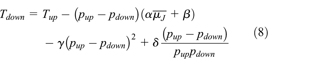
\begin{matrix} T_{down} = T_{up} - (p_{up} - p_{down}) (α \bar{μ_{J}} + β) \\ - γ {(p_{up} - p_{down})}^{2} + δ \frac{(p_{up} - p_{down})}{p_{up} p_{down}} \end{matrix}

(8)

where α, β, γ, and δ are empirical coefficients. The values of α, β, γ, and δ are 3.869, 4.9654 × 10⁵, 1.6 × 10¹⁴, and 1.3 × 10⁻⁶, respectively

\bar{μ_{J}} = \frac{1}{C_{p}} \frac{- \bar{p} b {\bar{v}}^{3} + 2 a {\bar{v}}^{2} - 3 ab \bar{v}}{\bar{p} {\bar{v}}^{3} - a \bar{v} + 2 ab}

(9)

\bar{p} = \frac{p_{up} + p_{down}}{2}

(10)

For air, the values of a and b are 0.1358 and 0.0000367, respectively.

Substituting equation (10) into equation (1) yields

\bar{v} = f (T_{1}, \bar{p})

(11)

where p_up and T_up are the pressure and temperature before throttling, respectively, and p_down and T_down are the pressure and temperature after throttling, respectively.

Dynamic model of the CAE

In the actual working process, the supply pressure of the CAE is lower than the critical pressure p_c, so the air in the CAE is considered to be an ideal gas. The thermodynamic model of the CAE has been introduced in author’s previous work.²⁵ The following equation, derived from Newton’s principle for a rotating body, describes the dynamics of the CAE. Figure 4 shows a model of the CAE coupled to a load. The following equation describes the dynamic system

T_{id} - T_{f} - T_{r} = J \overset{\cdot\cdot}{θ} + T_{L}

(12)

where T_id indicates the engine torque; T_f is the frictional torque; T_r is the reciprocating torque; T_L is the load torque; J is the moment of inertia of the crankshaft, flywheel, main gear, and rotating part of the connecting rod; and $\overset{\cdot\cdot}{θ}$ is the crankshaft angular acceleration.

Figure 4.

Engine and load model.

It has been suggested in the literature that the piston ring assembly may be the major component of the entire engine friction.²⁶ In this article, the friction torque includes two important components, one is piston ring assembly friction torque and the other is auxiliaries’ friction torque. The piston ring assembly friction torque is introduced in the author’s previous work.²⁵ The friction torque for auxiliaries including oil pump, generator, and gears from Zweiri et al.²⁷ is formulated as

T_{fa} = \sqrt{σ \overset{\cdot}{θ}}

(13)

where σ is the friction coefficient which is affected by oil temperature. In this article, the value of σ is considered as a constant value.

Simulation study and experimental verification

Simulation study of the APV

From the discussion above, it can be found that the performance of the APV is determined by many parameters. The major structural parameters of the CAE prototype are shown in Table 2.

Table 2.

Engine specifications and system parameters.

Type	Specification
Number of cylinders	1
Bore × stroke	88.0 mm × 89.0 mm
Crank-link rod ratio	0.316
Compression ratio	9.5
High-pressure tank pressure	10 MPa
Volume of high-pressure tank	50 L
Total heat transfer area of high-pressure tank	0.5 m²
Heat transfer coefficient of high-pressure tank	0.05 W m⁻² °C⁻¹
Buffer tank pressure	4 MPa
Volume of buffer tank	40 L
Heat transfer coefficient of buffer tank	1 W m⁻² °C⁻¹
Total heat transfer area of buffer tank	1 m²
High-pressure regulator sonic conductance	0.4 dm³ s⁻¹ bar⁻¹
Low-pressure regulator sonic conductance	3 dm³ s⁻¹ bar⁻¹
Load torque	30 N m

Besides the parameters listed above, the intake and exhaust cam profiles are shown in Figure 5. The maximum lift of the intake valve is 3.5 mm, and it opens at a crank angle of 0° and closes at 90°. The maximum lift of the exhaust valve is 5.7 mm, and it opens at a crank angle of 180° and closes at 355°.

Figure 5.

Intake and exhaust cam profiles.

Figure 6 depicts the power characteristics when the supply pressure is 2 MPa and the load torque is 30 N m. It can be seen that when the output torque is equal to the load torque, the output power starts to decrease slowly. The main reason is that the temperature of the intake compressed air drops during the working process. The various instantaneous engine torques lead to the output power fluctuation.

Figure 6.

Output torque and power curves with respect to time (s).

While running the dynamic system model, the following air temperatures were monitored: the high-pressure tank (indicated by T_hb), the outlet of the high-pressure regulator (indicated by T_ha), the low-pressure tank (indicated by T_lb), and the outlet of the low-pressure regulator (indicated by T_la). Figure 7 shows the simulated temperature curves when the set pressures of the high- and low-pressure regulators are 4 and 2 MPa, respectively. It is noted that the temperature dropped sharply during the working process.

Figure 7.

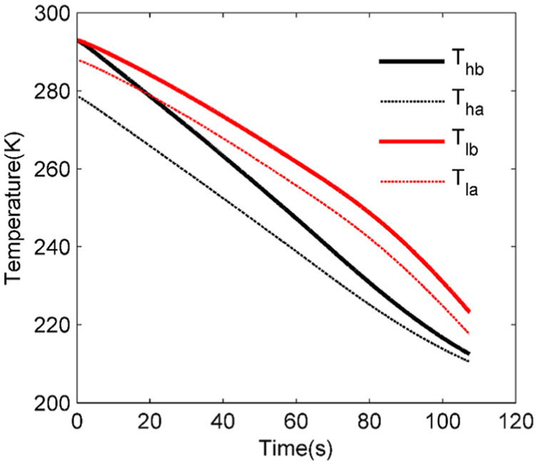
Curves of T_hb, T_ha, T_lb and T_la during the running process.

The pressure curves of the compressed air in the high-pressure and buffer tanks are shown in Figure 8. It is clear that the pressure of the high-pressure tank decreased dramatically during the working process. In contrast, the pressure of the buffer tank initially remained almost constant as time increased. However, at 80 s, the pressure of buffer tank started to decrease.

Figure 8.

Pressure curves of high-pressure and buffer tanks with respect to time (s).

The primary reason is that when the supply air flow is sufficient, the regulator is able to keep the pressure stable. If the supply pressure is insufficient, the regulator will not maintain pressure stabilization.

Figure 9 shows the rotating speed of the crankshaft during the working process. When the average output torque is equal to the load torque, the average speed tends to stabilize. However, it is clear that the rotating speed started to decrease slowly. That is because the energy of supply air continues decreasing as the temperature decreased.

Figure 9.

Speed curves with respect to time (s).

Experimental setup

The experiment was setup (as mentioned earlier) to verify the mathematical model. The experimental apparatus, as shown in Figure 10, consists of a high-pressure tank (made of carbon-fiber material), a high-pressure regulator (CONCOA 400 series regulator), a buffer bank, a low-pressure regulator, a flow meter, a CAE, a starter that drives the engine if the intake valve is not open at initial startup, a data acquisition system, a torque transducer (TPS-A-100NM), and an electromagnetic brake. Figure 11 shows a picture of the experimental setup.

Figure 10.

Experimental setup of the air-powered vehicle system test rig.

Figure 11.

Photograph of the experimental compressed air engine setup.

Before the experiments, 30 MPa of compressed air was stored in the high-pressure tank, and the prototype of the CAE was designed, as shown in Figure 1. The details of the prototype have been published in prior work.²⁵ The low-pressure regulator adjusted the pressure of the compressed air stored in the buffer tank for various experimental conditions. The flow meter provided air flow under normal operating conditions. The test bench included a 100-N m torque transducer, combined with an electromagnetic brake to measure the power output from the test engine. The electromagnetic brake applied a load varying from 0 to 100 N m. All data from the experiments were transferred to the data acquisition unit for recording and further analysis.

Experimental results

The efficiency of the CAE is defined as the ratio of the output shaft energy to the input energy²⁵

η = \frac{W}{E}

(14)

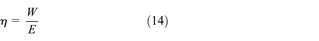
The output shaft energy can be expressed as

W = P_{e} t

(15)

where

P_{e} = \frac{T_{out} n}{9550}

(16)

where T_out is output torque of the APV system, n is the output speed of the APV system, and t is the running time.

According to Cai et al.,²⁸ the available energy of the compressed air can be calculated as follows

E = p_{a} V_{a} \ln \frac{p_{s}}{p_{a}}

(17)

where p_a is the atmospheric pressure, V_a is the normal volume, and p_s is the pressure of the supply air.

The method presented in an earlier section was applied, and the speeds were set from 860 to 260 r min⁻¹ by adjusting the electromagnetic brake. The supply pressure was set at 2 MPa, and the energy efficiency and torque of the APV system was graphed with respect to speed. These are shown in Figure 12.

Figure 12.

Torque and efficiency curve with respect to speed.

As shown in Figure 12, it is clear that the trends of the output torque and efficiency change between the simulation and experimental results are consistent. Therefore, the mathematical model has a good reference value for estimating the performance of the real APV system. However, there are two differences between the simulation results and the experimental results: (1) the values of output power and efficiency in the simulation results are greater than the experimental results, and (2) the error between the experimental results and the simulation results increases with the increase in speed.

The main reasons for the differences are summarized as follows:

The simulation is based on the assumption that no leakage occurs during the working cycle. However, in the actual process, leakage at the exhaust and intake valves is difficult to avoid.

Some practical frictional torques, such as those from bearings, the valve train, and pumping losses, are neglected in the mathematical model. As a result, the values of the simulation results are larger than the experimental results.

In the mathematical model, the oil viscosity is considered to be a constant value. However, in fact, the oil viscosity, as a function of temperature and pressure, is typically determined by a nonlinear least-squares method for exponential functions.²⁷

As the speed increases, the oil pressure increases. The relationship between the oil pressure and speed is shown in Figure 13. It is obvious that as the oil pressure increases, more torque is consumed by the fuel pump. The fuel pump is not considered in this simulation.

Figure 13.

Oil pressure curve at different speeds.

Other uncontrollable factors in the experiment, such as fluctuations in the supply pressure, mechanical efficiency, and atmospheric temperature, are also reasons for the differences between the simulation and experimental results.

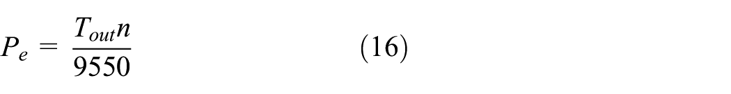
The gas loss rate is defined as the ratio of the mass of supply gas to the output power

g_{e} = \frac{ρ Q_{a}}{P_{e}}

(18)

where Q_a is the flow rate under normal conditions, ρ is the gas density, and P_e is the output power.

Figure 14 shows the relationship between the output power and gas loss rate with respect to speed at different supply gas pressures.

Figure 14.

Output power and gas loss rate with respect to speed.

As shown in Figure 14, the highest output power can be obtained when the speed is approximately400 r min⁻¹. The lowest gas loss rate can be obtained at the lowest speed. When the speed is >600 r min⁻¹, the gas loss rate increases rapidly. In the actual process, the APV system may have obtained better efficiency at lower speed. However, speed fluctuations increased with decreasing speed during the running process. Therefore, the speed of the CAE should be controlled within a certain range.

The CAE stopped at approximately 5.8 mA. When the electric current reached 9 mA, the air control valve opened fully. The experimental results between I and the speed of the CAE are approximated by the polynomial curve (y), as shown in Figure 15. The electric current (I) either increased or decreased linearly by controlling the unit with the following cycle: 5.8 → 9 → 5.8 mA (within a 2-s period). In fact, the polynomial curve can be used as a control function, and in the following section, it is converted to a transfer function.

Figure 15.

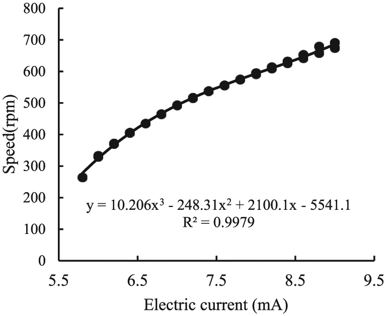
Relationship between the electric current I and the speed.

Fuzzy control design

The experimental results show that the control speed and supply pressure are important parameters to improve the APV system performance. When the external load decreases, the supply pressure is adjusted to maintain a steady speed. To improve the performance, we implemented fuzzy logic with a proportional–integral–derivative (PID) control scheme for the APV system. The PID control diagram is shown in Figure 16. First, we tried to select the best parameters for the PID controller based only on the error and its integration, as described by equation (19)

u (t) = k_{p} e (t) + k_{i} \int e (t) d τ + k_{d} \frac{de (t)}{dt}

(19)

Figure 16.

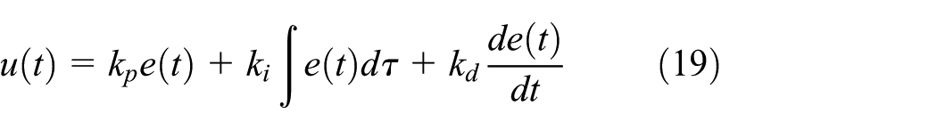
Fuzzy PID control diagram.

The selections of k_p, k_i, and k_d vary for different external loads. Hence, we implemented the fuzzy logic control to improve the system performance. Initially, large values of k_p, k_i, and k_d were required to have enough control power in overcoming static friction and improving the transient response. After the transient period, the values of k_p and k_i were decreased to maintain a good performance at the steady-state stage. The switching rules on the k_p, k_i, and k_d are based on the following fuzzy inference rules

\begin{matrix} IF E belongs to {\tilde{S}}_{Ei} AND EC belongs to {\tilde{S}}_{Ci} \\ THEN {\tilde{k}}_{p} belongs to {\tilde{S}}_{kp}, {\tilde{k}}_{i} belongs to {\tilde{S}}_{ki}, \\ AND {\tilde{k}}_{d} belongs to {\tilde{S}}_{kd} \end{matrix}

(20)

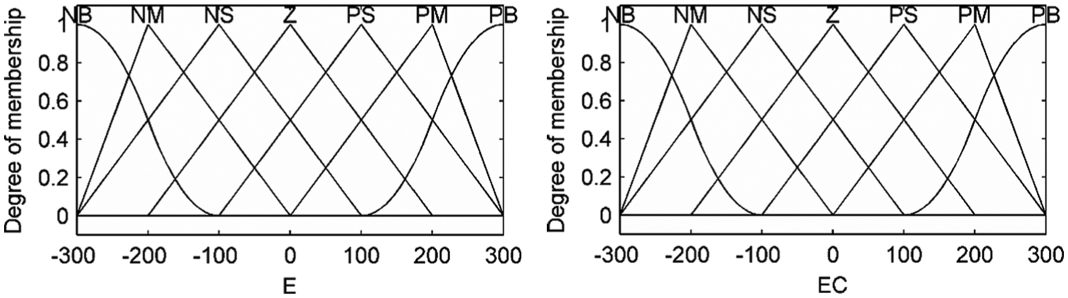
where E and EC represent error and its variation rate, respectively. ${\tilde{S}}_{Ei}$ and ${\tilde{S}}_{Ci}$ represent the corresponding fuzzy sets. ${\tilde{k}}_{p}$ , ${\tilde{k}}_{i}$ , and ${\tilde{k}}_{d}$ represent the corresponding fuzzy variables of k_p, k_i, and k_d. Their corresponding fuzzy sets are represented as ${\tilde{S}}_{kp}$ , ${\tilde{S}}_{ki}$ , and ${\tilde{S}}_{kd}$ . The fuzzy membership functions for the error E are shown in Figure 17. The notation in this figure, such as NL, NM, NS, PS, PM, PL, and ZE, represents the fuzzy sets which represent “negative large,”“negative middle,”“negative small,”“positive small,”“positive middle,”“positive large,” and “no error.”

Figure 17.

Fuzzy of membership functions for the error E and the error rate EC.

According to the experimental results, the speed ranges from 300 to 500 r min⁻¹. The response of the system under different speeds is shown in Figure 18. It is obvious that fuzzy PID control has a good control effect.

Figure 18.

Fuzzy PID control.

Conclusion

In this article, an APV was introduced. Simulations and experimental studies of the APV were performed, and the conclusions are summarized as follows:

The trends of the output torque and efficiency from the simulation results are consistent with the experimental results. The mathematical model has a good reference value in estimating the performance of the real APV system.

The highest output power 1.92 kW can be obtained when the supply pressure is 2 MPa, and the speed is 420 r min⁻¹. The lowest gas loss rate can be obtained at lowest speeds.

To obtain a stable speed and a good economic performance, the speed of the prototype should be controlled between 300 and 500 r min⁻¹.

The fuzzy control has a good control effect. The actual speed stabilizes quickly and reaches the desirable speed.

Footnotes

Academic Editor: Amir Alavi

Declaration of conflicting interests

The author(s) declared no potential conflicts of interest with respect to the research, authorship, and/or publication of this article.

Funding

The author(s) disclosed receipt of the following financial support for the research, authorship, and/or publication of this article: This work was supported by the Foundation of Beijing Municipal Science and Technology Commission.

References

Wesseling

Faber

Hekkert

MP.

How competitive forces sustain electric vehicle development. Technol Forecast Soc 2014; 81: 154–164.

Uherek

Halenka

Borken-Kleefeld

. Transport impacts on atmosphere and climate: land transport. Atmos Environ 2010; 44: 4772–4816.

Shancita

Masjuki

Kalam

. A review on idling reduction strategies to improve fuel economy and reduce exhaust emissions of transport vehicles. Energ Convers Manage 2014; 88: 794–807.

Raj Singh

Singh

. A study of performance output of a multivane air engine applying optimal injection and vane angles. Int J Rotat Mach 2012; 2012: 578745.

Szabłowskia

Milewskia

. Dynamic analysis of compressed air energy storage in the car. J Power Technol 2011; 91: 23–36.

Chen

Ding

. Air fuelled zero emission road transportation: a comparative study. Appl Energ 2011; 88: 337–342.

David Huang

Tzeng

S-C

. Development of a hybrid pneumatic-power vehicle. Appl Energ 2005; 80: 47–59.

David Huang

Tzeng

S-C

W-P

. Hybrid pneumatic-power system which recycles exhaust gas of an internal-combustion engine. Appl Energ 2005; 82: 117–132.

Shaw

J-J

Chieh

Design of a hydraulic motor system driven by compressed air. Energies 2013; 6: 3149–3166.

10.

Singh

. Necessity and potential for bio-diesel use in India. In: Proceedings of the international conference on bio-fuel vision-2015, Bikaner, India, 13–15 October 2006, pp.71–84.

11.

Singh

Development of a vaned-type novel air turbine. Proc IMechE, Part C: J Mechanical Engineering Science 2008; 222: 2419–2426.

12.

Shen

Y-T

Hwang

Y-R.

Design and implementation of an air-powered motorcycles. Appl Energ 2009; 86: 1105–1110.

13.

Engineair Company. The solution to pollution, 2014, http://engineair.com.au/

14.

Huang

C-Y

C-K

C-J

. Experimental investigation on the performance of a compressed-air driven piston engine. Energies 2013; 6: 1731–1745.

15.

Mistry Manish

Rathod

Sorathiya

. Study and development of compressed air engine-single cylinder: a review study. Int J Adv Eng Technol 2012; 3: 271–274.

16.

Chen

P-L

X-L

Liu

Simulation and experimental study electro-pneumatic valve used in air-powered engine. J Zhejiang Univ Sci A 2009; 10: 377–383.

17.

Chen

Zheng

. Study on real-gas equations of high pressure hydrogen. Int J Hydrogen Energ 2010; 35: 3100–3104.

18.

Ren

Yang

. Pneumatic performance study of a high pressure ejection device based on real specific energy and specific enthalpy. Entropy 2014; 16: 4801–4817.

19.

Luo

Wang

Exergy analysis on throttle reduction efficiency based on real on gas equations. Energy 2010; 35: 181–187.

20.

Saffari

Zahedi

A new alpha-function for the Peng-Robinson equation of state: application to natural gas. Chin J Chem Eng 2013; 21: 1155–1161.

21.

Berberan-Santos

Evgency

Pogliani

The van der Waals equation: analytical and approximate solutions. J Math Chem 2008; 43: 1437–1457.

22.

Cai

Shi

Dynamic heat transfer model for temperature drop analysis and heat exchange system design of the air-powered engine system. Energy 2014; 68: 877–885.

23.

Shi

Cai

Working characteristics of two kinds of air-driven boosters. Energ Convers Manage 2011; 52: 3399–3407.

24.

Jaime

The Joule–Thomson coefficient for pure gases and their mixtures. Chem Educat 1999; 4: 51–57.

25.

Cai

Shi

. Dimensionless study on efficiency and speed characteristics of a compressed air engine. J Energ Resour Technol 2015; 137: 044501.

26.

Zweiri

Whidborne

Seneviratne

LD.

Dynamic simulation of a single-cylinder diesel engine including dynamometer modelling and friction. Proc IMechE, Part D: J Automobile Engineering 2000; 213: 391–402.

27.

Zweiri

Whidborne

Seneviratne

LD.

Instantaneous friction components model for transient engine operation. Proc IMechE, Part D: J Automobile Engineering 2000; 214: 809–824.

28.

Cai

Kawashima

Kagawa

Power assessment of flowing compressed air. J Fluid Eng: T ASME 2006; 128: 402–405.

Fuzzy logic speed control for the engine of an air-powered vehicle

Abstract

Keywords

Introduction

Introduction of the air-powered vehicle system

Theoretical analysis

System simplification

Mathematical modeling of the APV system

Gas tank

State equation

Energy equation

Pressure regulator

Continuity equation

Joule–Thomson effect and the temperature change of throttle reduction

Dynamic model of the CAE

Simulation study and experimental verification

Simulation study of the APV

Experimental setup

Experimental results

Fuzzy control design

Conclusion

Footnotes

Declaration of conflicting interests

Funding

References