
Abstract
The links of the multi-closed-loop deployable mechanism are generally adjusted when being assembled, for the purpose of making the whole mechanism satisfy the requirements in fully deployed, folded, or the other key configurations. In order to calculate the appropriate adjustment amount, the complex adjustment amount of the whole mechanism is first defined by root mean square. And then, the adjustment model for planar mechanism involving different constraints is constructed according to the different situations. Through linearization of this model, it can be applied to calculate the adjustment sensitivity of this type of mechanisms. Second, with the factor of the practical adjustment in engineering, the three computation modes of adjustment (bidirectional adjustment, invariant adjustment, and unidirectional adjustment) have been developed. Furthermore, the multi-configuration adjustment approach has been proposed to make the assembled mechanism satisfy the requirements in different configurations. At last, all the above approaches in this article have been implemented in the scissor-like element mechanism and two-loop deployable mechanism. The achievement of this research provides a significant reference for assembling the multi-closed-loop mechanisms.
Introduction
The deployable mechanisms which can be extendable from a folded stowed configuration to an unfolded deployed configuration are widely utilized in the space antenna, solar array, and other applications. In order to increase the stiffness of these kinds of mechanisms, many deployable mechanisms, such as SEASAT-A, ERS-1, and Radarsat-2, are designed in the form of the multi-closed-loop structure.1–4 The research of the multi-closed-loop mechanism has been performed in a few of literatures and developed different kinds of these mechanisms. In 1990, Hoberman 5 invented an expandable and collapsible sphere toy which was constructed by numbers of the scissor-like elements (SLEs) in closed chains. Inspired by that, the more formation of a family of the planar parallelogram linkages were obtained by You and Pellegrino. 6 St-Onge and Gosselin 7 proposed a new family of deployable mechanisms composed by one degree of freedom (1 DOF) planar linkages. In addition, some researchers aroused the interest in several deployable Platonic mechanisms based on a single-looped dual-plane-symmetric spatial linkage, which was first published by Wohlhart. 8 And more ideas of synthesizing polyhedral linkages out of 8R linkages came out in Kiper, 9 Wei and Dai, 10 and Ding et al. 11 Besides the configuration design, the academic study also focuses on mobility analysis. Gantes 12 proposed a symbolic manipulation technique to perform the kinematic analysis of the foldable mechanism composed of particular elements. Patel and Ananthasuresh 13 developed a kinematic theory for radially foldable closed-loop linkages using the algebraic locus of the coupler curve. Liu and colleagues 14 discussed the deployment planar deployable support truss structure by means of the closed-loop equations and the Kane equation.
When manufacturing the mechanisms, the actual lengths of the manufactured links usually have a deviation from the nominal size. In manufacturing, the nominal size is a size “in name only” used for identification. 15 The dimension of the actual product may not match any nominal size, but within the domain of the proper tolerance the nominal size corresponds to. The deviations cause the degradation of the deployed accuracy, which sometimes result in the great distortion of the whole deployable mechanism. 16 To lower the distortion, we generally adjust the length of each link to fulfill the accuracy requirement when the whole mechanism is being assembled. However, the multi-closed-loop deployable mechanisms consist of numbers of rods, joints, and closed loops. Most deployable mechanisms include overconstraints, which make the accuracy analysis harder. The overconstraint conditions depend on the specific geometric constraints determined by the link length or joint angle, which is significant to the mobility and kinematics of the whole mechanism. If these geometric constraints cannot be conserved after the mechanism is assembled, the mobility may be changed. In order to guarantee the assembled mechanism still capable of motion from the folded configuration to the deployed configuration, the geometric relationship among these links should be carefully considered. In addition, the modes of adjustment in the practice field also have to be involved in the calculation since different modes generate different adjustment results. In order to obtain the appropriate adjustment amount, the accuracy analysis and adjustment method for this kind of mechanisms should be prior established. However, few literatures have been concentrated on the accuracy analysis, especially on the adjustment with high accuracy requirements. Hedgepeth 17 proposed an inverse frequency squared method to calculate the mean square of the surface error preliminarily. The evaluation of four different methods for estimating the surface error was presented in Mobrem. 18 Tang et al. 19 analyzed the surface accuracy of a large deployable antennas based on the stochastic finite element method. The above references were only concerned about the accuracy analysis of the mechanisms which are in the fully deployed configuration. A few of studies have been devoted to investigating the motion accuracy for the open-loop mechanisms or the parallel mechanisms. Pertile et al. 20 took a detailed accuracy analysis for a 3-DOF open-chain point mechanism. Wang and Ehmann 21 analyzed the accuracy of a Stewart platform by the utilization of a first- and second-order error models. Some researchers applied the equivalent kinematical model22–24 or the principle of virtual work25,26 to investigate the clearance effect. Because of large numbers of rods, joints, independent closed loops, and the arbitrary topology structure in the deployable mechanisms, the above analytical model or method would become more complicated and require large calculation if being directly applied to such kind of mechanisms. In addition, few literatures have recently investigated how to calculate the appropriate adjustment under specific conditions.
With the consideration that many deployable array mechanisms in the flight orbit mainly adopt the principle of planar mechanisms, the research of the accuracy problem is focused on the multi-closed-loop planar mechanisms in this article. We first define the complex adjustment amount of the whole mechanism by root mean square, and propose the adjustment potential energy. Based on the minimum of the adjustment potential energy, a computation model is established, which is not only for the adjustment but also for the accuracy analysis. All the approaches are verified to be correct and feasible through the examples.
Basic adjustment model for planar mechanism
Mostly, the actual length of manufactured linkage is not equal with the nominal size as a result of manufacturing error and tolerance. When being assembled, the lengths of rods have to be adjusted by means of grinding or gasketing for the requirements of dimension chain, position precision, and so on. In this section, the basic adjustment model for the planar mechanism is studied based on the minimum of energy. For the planar binary links, suppose
In view of Figure 1, A and B are the locations of the two revolute joints in rod e.
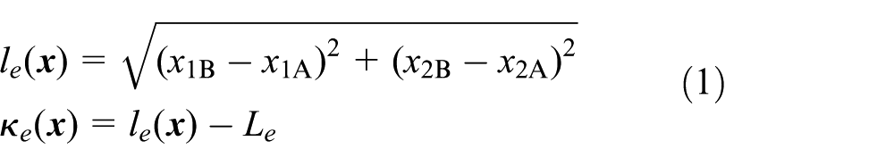

Dimension of rod e.
where

where b is the number of rods. In order to make the adjustment amount of the whole system as less as possible, it is hoped that the complex adjustment amount

Adjustment of rods by gaskets.
In order to solve the above problems, the adjustment weight
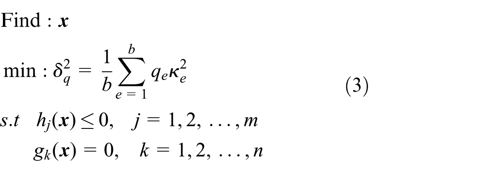
where
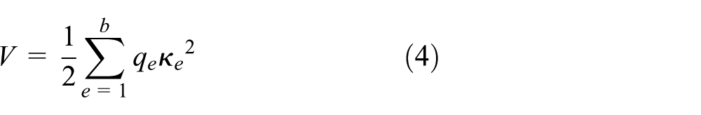
And the objective of equation (3) is equivalent to the following formula
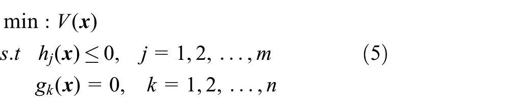
In view of the formula,
For resolving the optimization problem of equation (5), the objective can be expanded to the function

If the value of function

Assume

where p is the iteration number and
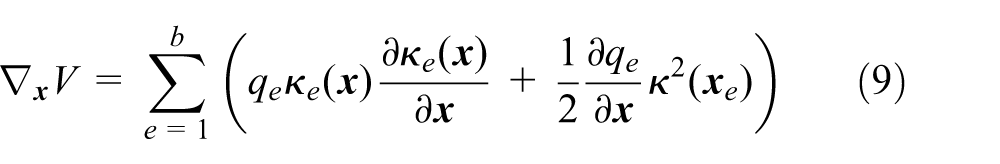
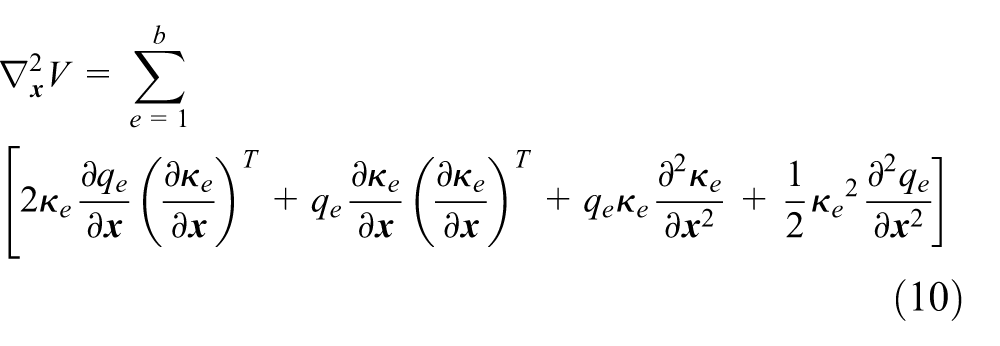
And the first- and second-order derivative of

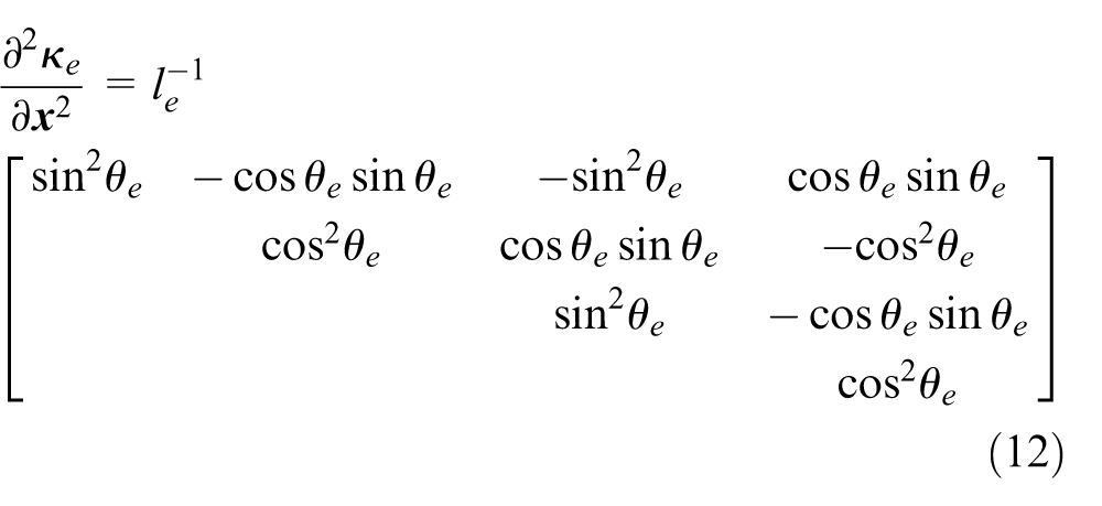
Equation (12) is referred to as the geometric stiffness matrix. 27 Through equations (9) and (10), the gradient vector and the second-derivative matrix can be formed. The solution of equation (8) provides the nodal coordinates of the assembled mechanism, and then the assembling lengths of the rods can be obtained through equation (1). Above all, the calculation procedure for the adjustment of the multi-closed-loop mechanism can be summarized as the following steps:
Step 1. Input the manufacturing lengths of the rods, give the weight
Step 2. Input the initial nodal coordinate vector
Step 3. Calculate the gradient vector, the Hessian matrix, and the constraint equations for each link.
Step 4. Assemble the gradient vector and the Hessian matrix of the whole mechanism, and substitute them into equation (8) to perform the iterative computation.
Step 5. If the convergence is achieved, the iteration is stopped. Then, output the nodal coordinates and the assembling lengths. Otherwise, go to step 3 to continue the calculation.
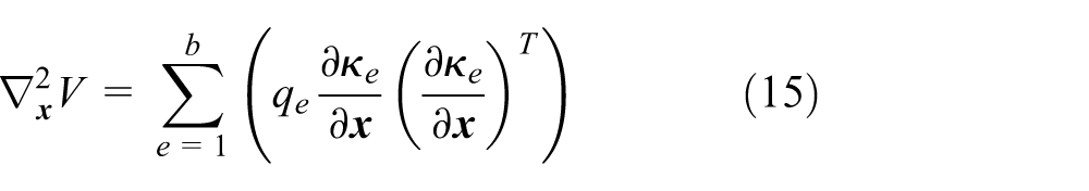
In the event that the adjustment amount of the rods is small, it generates the small distortion in the whole mechanism. The above nonlinear problem can be linearized. Let

In this case, the first term on the left of equation (13) can be approximately calculated by the theoretical coordinates. The weight

Equation (13) can be applied to investigate the sensitivity of the multi-closed-loop mechanism. Differentiating equation (13) with respect to the deviation

From the above equation, the sensitivity of the nodal displacements to the adjustment amount of each rod can be calculated. If the constraint

Using the sensitivity information, we can figure out which rod has the most influence on the accuracy, and which needs to be mainly concerned in the assembling procedure. Furthermore, we can use the sensitivity information to estimate the variation caused by the adjustment amount of each rod.
Overconstraint conditions
In a multi-closed-loop deployable mechanism, there possibly exist some overconstraints. Figure 3(a) is a 6R parallelogram mechanism where the specific geometric constraints are AB = CD = EF and AB∥CD∥EF. Obviously, this mechanism includes overconstraints. If the specific relationships are not satisfied, the motion of the mechanism is unavailable as shown in Figure 3(b). Therefore, the specific geometric relationships have to be added to equation (8) as the optimization constraints in this situation.

6R parallelogram mechanism: (a) movable and (b) unmovable.
Modes of adjustment
In practical adjustment, there are three modes need to be concerned, which are bidirectional adjustment, invariant adjustment, and unidirectional adjustment.
Bidirectional adjustment
The bidirectional adjustment means that the rod can be modulated its length in both directions, that is, extension and shrink. To realize it in the calculation, the adjustment weights of the rods are set as a fixed uniform value, which makes the rods possess the same “stiffness” in both directions. Consequently, the rods are capable of varying their lengths in both directions during the calculation.
Invariant adjustment
When being assembled, it is sometimes hoped that the lengths of some specific rods are not changed. There are two ways to handle this problem. One way is to set a heavy weight (much larger than the other rods) to the specific rod. It makes the specific rod possess a “higher stiffness” in the optimization calculation. Another way is to regard the invariant rod as a length constraint in the calculation. The length constraint can be written as follows

Two ways are feasible to solve this problem.
Unidirectional adjustment
During the assembling procedure, the gaskets are usually utilized to change the assembling length of rod, as shown in Figure 2. In this situation, the rods can be only extended but not shrinked along its axis. Herein, we call it unidirectional adjustment.
From the above section, it is well known that the result of the adjustment calculation depends on the property of
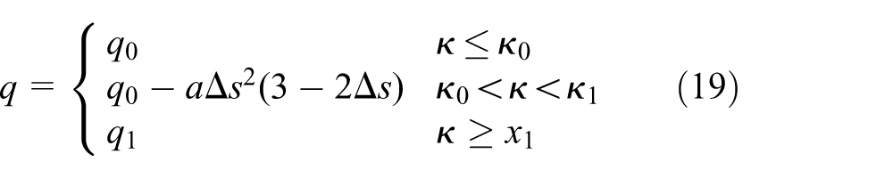
where
Through changing the distance between
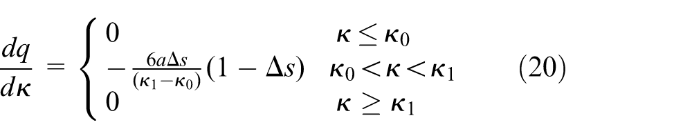
And the second-order derivative is
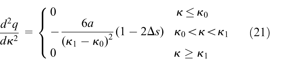
Equations (9) and (10) require the first and second derivatives of q with respect to
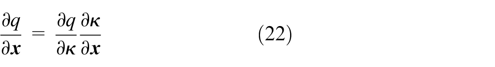
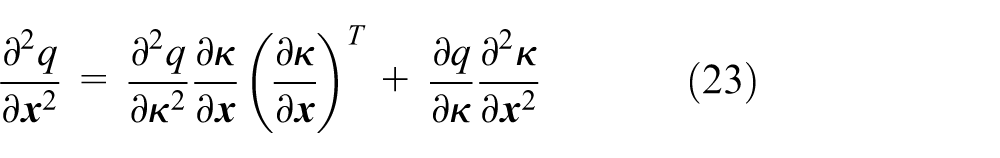
Substituting equations (11), (12), (20), and (21) into the above equations, the first and second derivatives of q with respect to
Adjustment in multi-configuration
The two configurations, that is, fully deployed and folded configurations, are significant for the deployable mechanisms. Figure 4 is a two-closed-loop mechanism extracted from Radarsat Extendable Support Structure (ESS). The auxiliary rods without influence upon the mobility of this mechanism are removed. The solid lines and dot lines represent the theoretical model and the practical assembly model, respectively. The rods of this mechanism are adjusted only according to the constraints in the deployed configuration as shown in Figure 4(a). When this mechanism is assembled and folded, the rods 3, 4, and 5 exceed out of the envelope as shown in Figure 4(b).
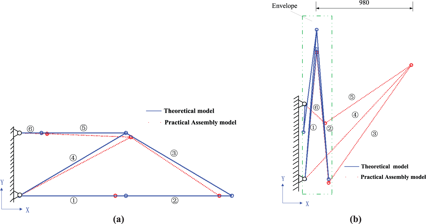
Assembly model in two configurations: (a) fully deployed configuration and (b) fully folded configuration.
Obviously, this result cannot be applied to the practical adjustment. To avoid that, it should be guaranteed that the deployable mechanism after being adjusted must satisfy the requirements in both configurations. For fully deployed configuration, it is mainly concerned about the surface accuracy because the low accuracy results in the degradation of the antenna performance. For the fully folded configuration, it is mainly concerned about the stowed position of mechanism. If the practical stowed position is far away from the theoretical one, the mechanism has risk of excess of the given envelope or interference with other objects. These requirements in the multi-configuration can be regarded as the constraints in the calculation.
Suppose

For the same mechanism, the length of individual rod in different configuration is always identical after being adjusted, which yields to the following equation

We regard the sum of multi-configuration adjustment potential energy (

On the right-hand side of equation (26), the first term represents the sum of multi-configuration adjustment potential energy,
Adjustment of SLE mechanism involving overconstraints
The SLEs are widely adopted to design the deployable mechanisms. 28 This type of deployable mechanisms is the pairs of rods connected to each other through a revolute joint, while at the same time, their end points are hinged to the end points of other SLEs. The geometric design results in zero stress in the deploying process. Figure 5 is a flat pantographic deployable mechanism, which obviously includes several overconstraints.
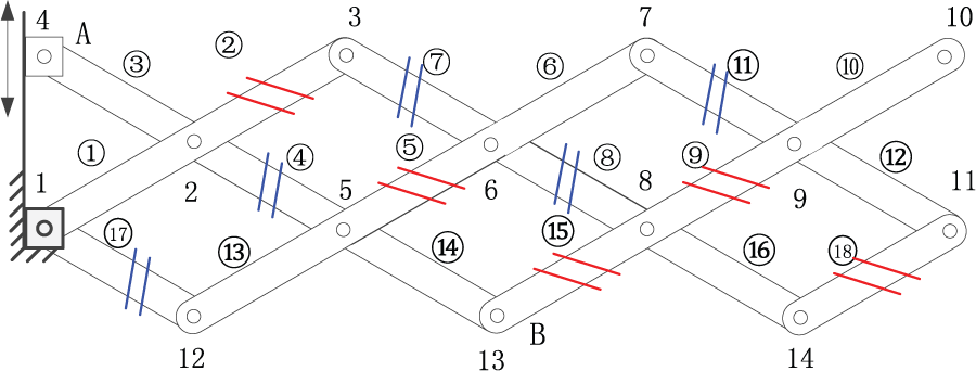
SLE mechanism involving overconstraints.
In Figure 5, the long rod (e.g. rod AB) can be regarded as the composition of some small rods (e.g. rods 3, 4, and 14). In order to make this mechanism move with zero stress, the overconstraints need to satisfy the following

The nominal and manufacturing length of individual rod are displayed in Table 1.
Nominal and manufacturing length of SLE mechanism.

Due to the manufacturing error, the rods have to be adjusted for assembling. Within the consideration of the rod fabrication, the distances between nodes 2 and 5, 5 and 6, 6 and 8, and 8 and 9 are difficult to be changed. The lengths of rods 4, 5, 8, and 9 are regarded as invariant, and these constraints can be written as follows

In calculation, in order to make the above rods invariant, the “stiffness” of these rods is set to be a higher weight. Herein, we give the weight of the invariant rods 1000 times as large as the other rods. Except from the invariant rods, the other rods are allowed to be adjusted in both directions and the weights of the other rods are all set as 1.0. Through the procedure in section “Basic adjustment model for planar mechanism,” the result can be calculated.
In Table 2, the positive sign of the adjustment amount means that the rods are extended when being adjusted, while the negative sign means the rods are shrinked. From Table 2, it is found that the adjustment amounts are very tiny in rods 4, 5, 8, and 9 because the weights of these rods are set much heavier than the other ones. It can also be concluded the following features of the lengths of the rods after being adjusted

Assembling length and adjustment amount of SLE mechanism.

These results are consistent with equations (27) and (28). Figure 6 shows the differences between the assembled mechanism and the theoretical mechanism. The adjustment amount of each rod presents in the closed box. The practical assembled mechanism is represented by the colorful ribbons and the theoretical mechanism is represented by the solid lines. We make the deviation between them scale up to make it clearly in the figure. The maximum deviation locates in node 10.

Difference between assembly mechanism and theoretical mechanism.
To prove that the adjusted mechanism is available to motion, the kinematic simulation is performed. Figure 7 provides the nodal trajectories of this mechanism in the deploying procedure. The dot slash lines are the trajectories of the joints, and the solid lines are the folded and deployed configurations. The nodal trajectories show that the movement is continuous and smooth, and demonstrate that the overconstraints are conserved by means of this adjustment approach.

Trajectories in deploying procedure.
Adjustment of two-loop deployable mechanism in multi-configurations
Figure 8 presents a multi-closed-loop deployable mechanism which is assembled in series by two identical two-loop deployable mechanisms (TLDM) described in Figure 4. 14 This assembly mechanism is composed of 12 rods, 4 closed loops, and capable of 4 DOFs. We call it 2-TLDM in this article.

Different configurations of 2-TLDM: (a) fully folded configuration, (b) fully deployed configuration, and (c) middle configurations when α 1 = 20° and 40°.
To achieve the complete deployment, there are four actuators equipped in this mechanism. The actuators M1, M2, M3, and M4 are located in nodes 1, 2, 3, and 7, respectively. M1 drives rod 1 to rotate with rod 13, and M2 drives rod 2 to rotate with rod 1. M3 and M4 rotate rods 7 and 9 with rods 2 and 7, respectively. When the mechanism is deploying, the angular velocities satisfy

The antenna surfaces are mounted on the rods 1, 2, 7, and 9. Therefore, their length is undesirable to be changed. This constraint can be written as follows

When the mechanism is fully deployed, the joints located between rods 1 and 2, rods 7 and 9, rods 5 and 6, and rods 11 and 12 are all locked. And the deployed angle


When the mechanism has been fully folded, the angles


where

where

The nominal and manufacturing length of each rod can be expressed in Table 3. The maximum absolute deviation of these rods is 115.6 mm. In this section, two modes are adopted, that is, bidirectional and unidirectional adjustments, to calculate the adjustment amount of this mechanism and validate the feasibility of the above method.
Nominal and manufacturing length of 2-TLDM.

2-TLDM: two-loop deployable mechanism.
Bidirectional mode
In this mode, the adjustment weight of each rod

2-TLDM adjustment in bidirectional mode.

2-TLDM: two-loop deployable mechanism.
From Table 4, the adjustment amount of rods 1, 2, 7, and 9 are zeros because of the setting of heavy weights on these rods. It is also noticed that rods 3 and 6 have the larger adjustment percentage than the other rods in this case. The two deployed angles

Since the virtual spring model is added to the calculation, the maximum X-axis deviation of nodes 4, 5, 9, and 10 is only 9.3 mm when the mechanism is in the fully folded configuration. The maximum deviation of nodes 4 and 9 is 33.9 mm in the middle configurations. Compared with the whole mechanism size, these position deviations are relatively small. The fully deployed configuration in this adjustment mode is presented in Figure 9, where the solid lines describe the theoretical model, and the colorful ribbons describe the result of bidirectional adjustment. The adjustment amounts display in the nearly boxes. The maximum position deviation between them locates on node 4.

Fully deployed configuration in bidirectional adjustment mode.
Unidirectional mode
In this mode, the rods can be only extended but not shrinked along its axis. The adjustment weight of each rod
2-TLDM adjustment in unidirectional mode.

2-TLDM: two-loop deployable mechanism.
From Table 5, the adjustment amount of rods 1, 2, 7, and 9 are very close to zeros. And rod 3 has the much larger adjustment amount and percentage than all the other rods in this case. The

Owing to the virtual spring model, the coordinates of nodes 4, 5, 9, and 10 are almost equal with the theoretical ones in X-axis in the fully folded configuration. The maximum deviation of nodes 4 and 9 is 10.6 mm in the middle configurations. Figure 10 presents the fully deployed configuration in the unidirectional adjustment mode. The solid lines represent the theoretical model and the colorful ribbons represent the result of unidirectional adjustment. And the maximum position deviation appears on node 4.

Fully deployed configuration in unidirectional adjustment mode.
The adjustment amounts of the two modes are plotted on the bar chart as shown in Figure 11. Compared with these two results, the adjustment amount in unidirectional mode is either positive or zero, which satisfies the requirement of the unidirectional mode. The complex adjustment amount

Adjustment amount in two modes.
To prove that the adjusted mechanism can move, the kinematic simulation is performed. We examine the trajectories of nodes 4 and 9. In Figure 12, the red dot lines describe the nodal trajectories of the nominal model; the blue dot slash lines describe the trajectories of the bidirectional adjustment and the black lines describe the trajectories of the unidirectional adjustment. The red crosses represent the control points when
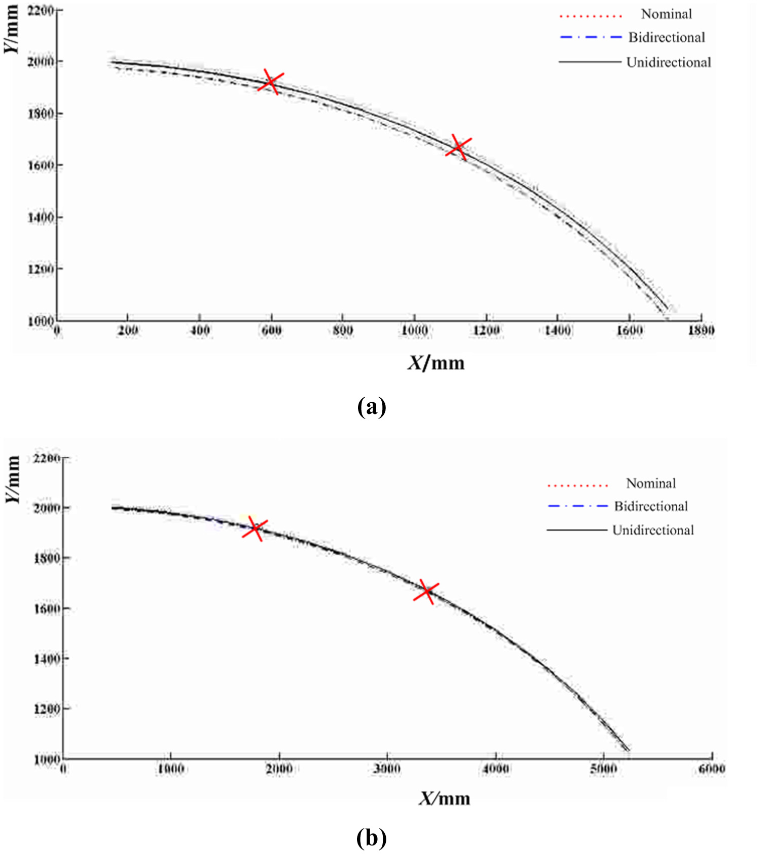
Trajectories of 2-TLDM nodes: (a) node 4 and (b) node 9.
Adjustment sensitivity analysis
From section “Basic adjustment model for planar mechanism,” it is known that if the deviation of rods is small, the above nonlinear problem can be linearized to equations (13), (16), and (17), which can be used to analyze the adjustment sensitivity of the multi-closed-loop deployable mechanism in this section. Take the 2-TLDM for instance, when the mechanism is in the deployed configuration, the deployed angles
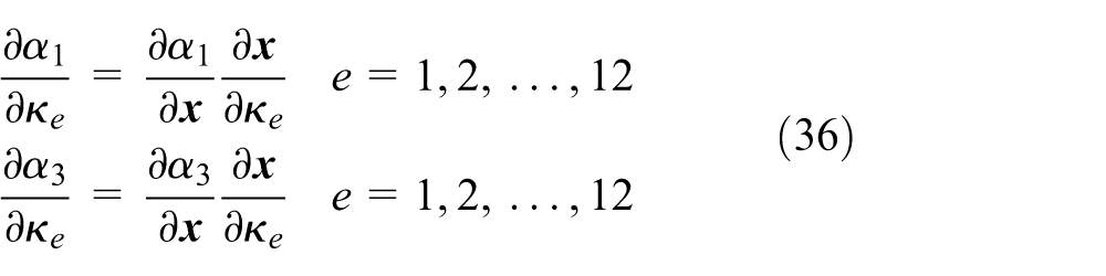
where
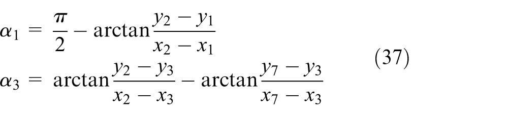
In equation (36),
Sensitivities of

In Table 6, the sensitivities of
Assume

From the above equation, the adjustment amount of each rod can be preliminarily obtained within a small range.
From section “Adjustment in multi-configuration,” it is well known that the mechanism of the stowed position has also to be considered. In this section, we calculate the sensitivity of

Sensitivity of
Figure 13 demonstrates that the sensitivities are greatest in the fully folded configuration. As the mechanism is deploying (

The adjustment sensitivity reveals the relationship between the variation of the whole mechanism and the adjustment amount of each rod. Through equation (17), the sensitivity information is obtained. And then, the variation of the key point index, such as deployed angle or folded position, can be calculated and the adjustment amount of each rod would be preliminarily estimated, which in turn reduce the time and the cost, and is very useful in the assembling procedure.
Conclusion
The multi-closed-loop planar deployable mechanism comprises large numbers of rods, joints, closed loops, and the overconstraints. In this article, the complex adjustment amount
All the approaches mentioned above have been implemented in the SLE mechanism and 2-TLDM. The kinematic simulation shows that the movements of the adjusted mechanisms are continuous and smooth, and the nodal trajectories are extremely closed to the control points from the theoretical model. The linear model has been utilized to analyze the adjustment sensitivity of 2-TLDM. And the most significant sensitivity has been identified. This research will help to reduce the difficulty and the cost of assembling the multi-closed-loop deployable mechanisms.
Footnotes
Academic Editor: ZW Zhong
Declaration of conflicting interests
The author(s) declared no potential conflicts of interest with respect to the research, authorship, and/or publication of this article.
Funding
The author(s) disclosed receipt of the following financial support for the research, authorship, and/or publication of this article: This project is supported by the National Natural Science Foundation of China (Nos 51305271, 61233010, 51105013, and 61305106).