Springback prediction of three-dimensional variable curvature tube bending

Abstract

The springback phenomenon of tube bending occurs consequentially after unloading, which will affect the manufacturing accuracy and processing efficiency of the tubular products. In this article, the bending and springback processes of minor-diameter thick-walled tube are simulated by ABAQUS to reveal the springback laws. The springback prediction of three-dimensional variable curvature bent tube is projected on each discrete osculating and rectifying plane, and then the three-dimensional problem can be transformed into two dimensions. The mathematic relationship of the radius before and after springback in the plane is built by approximate pure bending springback experiments. The springback on such planes is transformed into three dimensions. The tube axes are merged by first-order geometric (G1) continuity and then compensated with the modified function according to the axis complexity, so as to establish mathematic analytic model for springback prediction of three-dimensional variable curvature tube bending. Finally, the feasibility, reliability, and accuracy of the model are verified by finite element method and experiments.

Introduction

With the industrial development, more and more high-strength, lightweight, and high-precision complex is required. Tubular products are widely used in many fields such as aeronautics and aerospace, shipbuilding, automobile, construction, pressure vessel, medical apparatus, and oil and chemical industries.^1,2 Tube-forming components have many desirable features, such as saving materials, reducing the weight, strengthening the structure, and absorbing the impact energy and shock. However, the defection of springback often occurs during the process of bending tube parts, which results in more complex geometric and higher shape accuracy requirements. It will affect the connectivity between components, sealing, and internal structure of products. A die surface design requires accurate springback prediction of tube bending, which can improve accuracy, shorten production cycle, and reduce costs of products.

As the shape of tube parts becomes more and more complex, three-dimensional (3D) configuration tube, which has changed curvature, has been widely utilized.^3,4 This 3D configuration tube is bended in 3D variable curvature, that is, the curvature of bended tube axis is not constant, and torsion is not identically zero.

The uneven plastic bending deformation of this kind of bent tube with variable curvature can strengthen the geometric nonlinearity and boundary nonlinearity, compared with constant curvature. And springback of 3D tube bending will raise new issues and challenges for the tube-forming technology.

Current research in springback of tube bending mainly focuses on the plane constant curvature axis tube with hot or cold bending, combined with advanced computer numerical control (CNC) tube-bending technology.^3,5,6 However, studies for 3D variable curvature bent tube have not been well developed, which are new challenges for the precision-forming technology.

According to the available literature, the research of 3D tube bending is focused on bending methods or processing equipment, but not much on springback. For example, a relatively novel bending technique “free-bending” is investigated with the aim of improving its applicability in the automotive industry. Free-bending permits bending in almost every geometry with different radii, bend-in-bends with only one die and without any reclamping of the tube or profile, and a finite element method (FEM) simulation model of the free-bending process was developed and verified using bending tests.^7,8 However, this method is also in a fledging period without deep research in springback. Three-roll-push-bending is another highly flexible manufacturing process for the production of 3D free-form bent tubes. And a finite element (FE) model which considers all of the relevant influences, such as the machine kinematics, the friction, and the machine stiffness, has been developed.^9–12 Springback occurs during the three-roll-push-bending process, but has not been quantified or modeled so far. A kinematic bending method known as torque superposed spatial (TSS) bending, which is flexible, continuous, and adaptive two-dimensional (2D) and 3D bending of profiles with symmetrical and asymmetrical cross sections, has been developed in IUL-TU, Dortmund. The important influencing factors on the bending accuracy were investigated and described by experiments, FE simulation, and a semi-empirical model.^4,13,14 There was a simple springback compensation system based on the elementary theory of bending for a 3D bent profile with two successive bending radii in two different bending planes. It is not a general 3D variable curvature form. A new flexible bending machine has been developed in Japan. When tubes are fed into the fixed and mobile dies, they are bent by shifting the relative position of the mobile die. A change of the expected bending shape will need no change in the tooling system but only a new definition of the motion of the active die and the length of the fed tube. The active die movements are controlled by a 6-degree-of-freedom (DOF) parallel kinematic mechanism (PKM) with hydraulic servo drive.^15,16 The main purpose is to make use of the PKM not only to achieve a complete motion along six axes but also to obtain a high dynamic motion of the bending machine. The presented methods provide new and useful approaches for processing the variable curvature tubes.

In recent years, analytic method and elastic–plastic FEM are two main methods used to analyze the springback of the tube-bending process.^17–19 The 3D tube-bending springback law can also be revealed by experiment and numerical methods. Accurate prediction of bending springback is prerequisite for controlling the springback, which will contribute to the development of precise variable curvature tube-bending technology.

Mechanical properties test of 0Cr18Ni9 tube

At present, most of the mechanical behavior studies are focused on the sheet metals. However, there are not many researches on the tube. Mechanical behavior between sheet and tube is different since they are fabricated with different manufacturing techniques. Hence, it is necessary to reconsider the mechanical properties of the tube materials under specific modalities.

Tube materials are of great variety and different properties; the springback of small-diameter thick-walled tube, whose diameter is less than 10 mm and the ratio of outside diameter to wall thickness is less than 20 mm, is a major defect contrasted with wrinkling, cracking, and cross-sectional distortion. This article focuses on springback prediction model of 3D variable curvature bending.

Tensile testing of the materials in a tubular state

In this study, mechanical properties of minor-diameter thick-walled tubes of steel 0Cr18Ni9 with $\varphi$ 3 mm × 1 mm were investigated through a uniaxial tension test.

Sample preparation

The section dimension of tubular specimen for uniaxial tension is shown in Figure 1, according to the GB/T 228-2002. ²⁰ Two solid bars were inserted at both sides of the tube for gripping.

Figure 1.

Tubular specimen dimension for uniaxial tension test.

Uniaxial tension test

Three effective tensile tests were carried out with an electronic universal testing machine (CSS-44100). Tensile strength was measured by automatic signal acquisition system. Displacements were obtained by a vertical extensometer, with the gauge length of 50 mm. The velocity of the test was set to be 3 mm/min at ambient temperature.

Table 1 lists the material parameters obtained by uniaxial tensile tests. The true stress–strain curves of three tests are presented in Figure 2. And the hardening behavior is used during the numerical simulation.

Table 1.

Mechanical parameters of the thick-walled tube of 0Cr18Ni9.

Young’s modulus, E (GPa)	Yield strength, ${\sigma }_{0.2}$ (MPa)	Ultimate strength, ${\sigma }_b$ (MPa)	Poisson’s ratio, $\mu$	Density, $\rho$ (kg/m3)	Elongation, $\delta$ (%)
160	834	1050	0.3	7.93 × 103	11.86

Figure 2.

True stress–strain curves.

Approximate pure bending springback test of tubes

During the tube-bending process, after unloading, an elastic recovery occurs due to the release of the elastic stresses. This elastic recovery is called springback. Springback is an important and decisive factor in obtaining the desired geometry of parts and design of corresponding toolings. Springback of plane bending tubes is always signified by the curvature variation or angle variation of the tube axis. Curvature of the bent tube axis is the rotation rate of tangent angle to arc length. A larger curvature corresponds to a greater axis bending degree.

As shown in Figure 3, the lines PA and PB, respectively, tangent at points A and B with arc AB.

Figure 3.

Geometric principle of measuring angle.

According to the geometric relationship, $\angle \mathrm{PAO}=90\circ$ , $\angle \mathrm{PBO}=90\circ$ , $\angle \mathrm{AOB}+\mathrm{APB}=80\circ$ , and $\angle \mathrm{CPB}+\mathrm{APB}=180\circ$ . Then, $\angle \mathrm{AOB}=\mathrm{CPB}$ is denoted by $\theta$ .

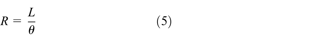
AD can be denoted by a, OA by R, and $\angle \mathrm{CAD}$ by ∂, then

$$\mathrm{AE}=a·\cos \partial$$

(1)

$$\mathrm{AP}=R·\tan \left(\frac{\theta }{2}\right)$$

(2)

$$\mathrm{DE}=a·\sin \partial$$

(3)

$$\tan \theta =\frac{\mathrm{DE}}{\mathrm{PE}}=\frac{\mathrm{DE}}{\mathrm{AE}-\mathrm{AP}}=\frac{a·\sin \partial }{a·\cos \partial -R·\tan \left(\frac{\theta }{2}\right)}$$

(4)

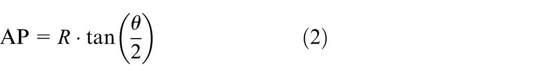
According to radius R and arc length L, the conversion formula is given by

$$R=\frac{L}{\theta }$$

(5)

The trigonometric function is given by

$$\tan \theta ·\tan \left(\frac{\theta }{2}\right)=\frac{1-\cos \theta }{\cos \theta }$$

(6)

$$\sin \partial ·\cos \theta -\cos \partial ·\sin \theta =\sin (\partial -\theta )$$

(7)

Scale line is shown in radians

$$\partial =\theta -\arcsin \frac{L·(1-\cos \theta )}{a\theta }$$

(8)

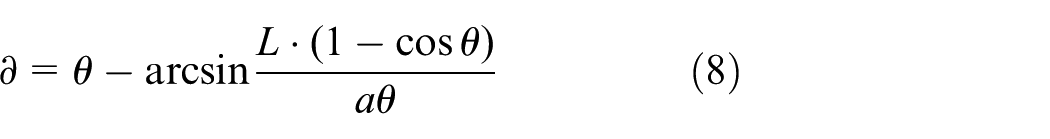
where ∂ is the radian of the scale line (rad), $\theta$ is the radian of the tube bending (rad), a is the radius of scale line (mm), and L is the arc length of the tube bending (mm).

Equation (8) can also be written in a more convenient format as follows

$$\theta =\partial +\arcsin \frac{L·(1-\cos \theta )}{a\theta }$$

(9)

The transcendental equation of $\theta$ has been established.

Figure 4 presents the experimental facility for the approximate pure bending springback test; with this test, the springback property with a certain radius can be obtained. Figure 5 gives the relationship of radii before and after springback; in this relationship, the radius after springback increases nonlinearly with the bending radius

$$y=0.000119x^3+0.027287x^2+0.423865x+5.617601$$

(10)

where y is the tube-bending radius after springback (mm); x is the radius before springback (mm), where x∈ [12.23, 72.60].

Figure 4.

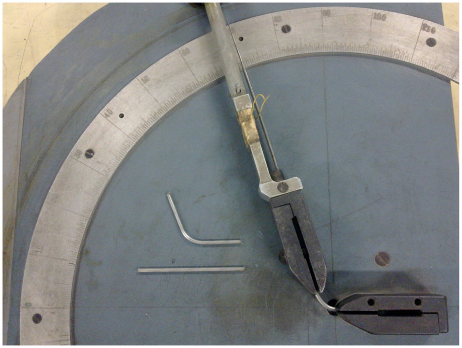
Measuring angle of approximate pure bending springback.

Figure 5.

Relationship of radii before and after springback.

Numerical simulation of 3D variable curvature tube bending and springback

FE model

Rotary-draw bending process of minor-diameter thick-walled circular tube is a complex forming process involving material nonlinearity, geometry nonlinearity, and boundary condition nonlinearity. To analyze these nonlinear behaviors effectively, a 3D elasto-plastic FE model for tube bending shown in Figure 6 is established by UG NX6.0 and ABAQUS 6.10.

Figure 6.

FE model of 3D variable curvature tube bending.

The thick-walled tube is modeled as a deformable body using eight-node linear brick, reduced integration, hourglass control, and solid element C3D8R. Advantage of higher accuracy of the results is solved, analytical precision is not significantly affected when the mesh distortion exists, and less prone to shear locking under bending load. The dies are modeled as rigid bodies using four-node 3D bilinear rigid quadrilateral element R3D4 to describe contact geometrical curved faces.

Among the methods of meshing, structured mesh can create rational dimension and good form meshes which are easily adapted and refined. The methods of local mesh refined are used to mesh the contact zone.

This study uses von Mises’ yield criterion. Table 1 presents the material properties used for the FE model. Surface-to-surface contact using penalty method is adopted in contacts between various dies and tubes. Coulomb friction model is employed, and the effect of relative velocity slipping on friction coefficient is negligible. The friction parameter is 0.1. Other simulation conditions are the same as the actual experiment conditions.

FE simulation of tube bending and springback

Analysis of boundary conditions

The trajectory of 3D variable curvature tube bending is a 3D space curve; for these complex boundary conditions, displacement loading programs, namely, real-time control of the 3D axis nodal displacement, are adopted during tube bending. The tangents of the axis discrete nodes are marked into vectors, and tube-bending load displacement trajectories are calculated by the tangential vectors of discrete nodes.

Select the axis of 3D variable curvature tube as the research object and the Frenet frame of the initial node of tube-bending axis as a reference to establish Cartesian coordinate system X–Y–Z. Then, the 3D variable curvature tube-bending process is simplified as variable curvature bending in the X–Y plane cooperating with Z displacement. The basic control method is shown in Figure 7, where plane I is the reference plane X–Y, and plane II is parallel to the X–Y plane:

1. OA _i rotates around Z-axis with O as the center in plane II, rotation angle is recorded as θ, and the length remains constant;

2. A _i B _i is the height of h_i and keeps Z-direction with node B _i moving though Z-axis;

3. B _i C _i is the length of l_i and keeps up with the tangent vector direction of the tube axis PC _i on the node C _i , with C _i moving though BC;

4. The included angle between OA _i and B _i C _i in the X–Y plane is recorded as φ;

5. The 3D variable curvature tube-bending process will be controlled by the angle θ, φ, the height of h_i, and so on.

Figure 7.

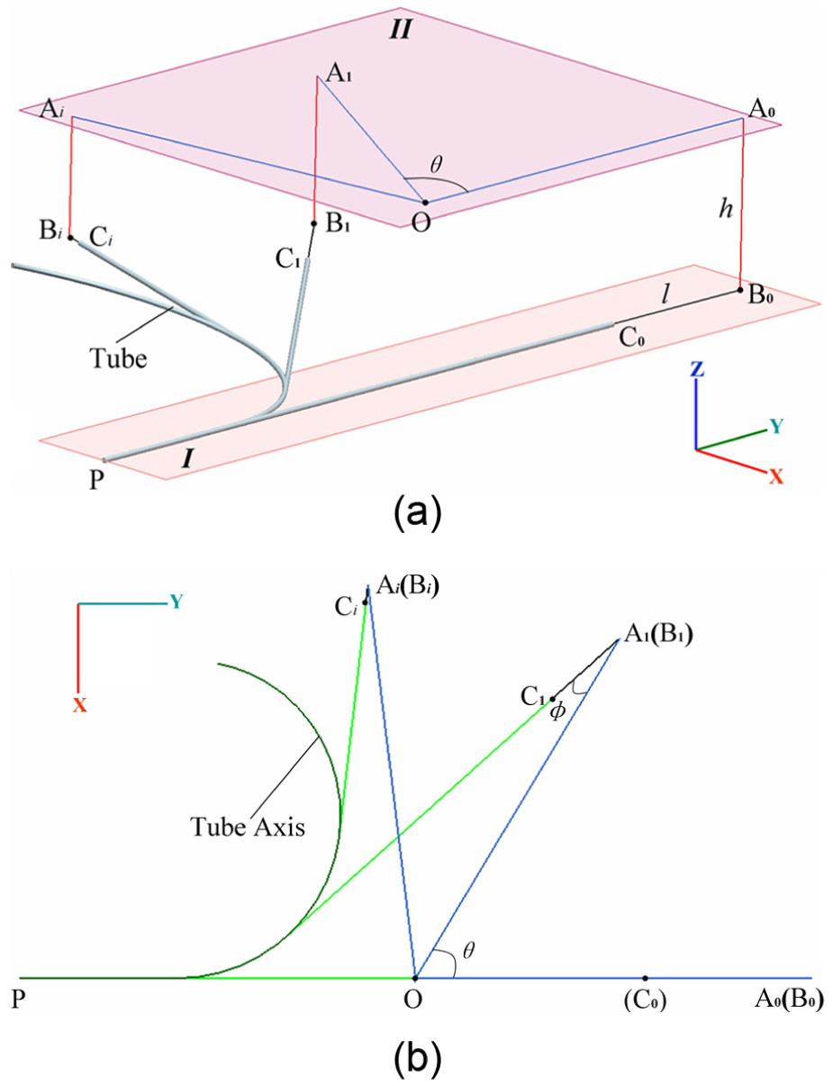
Rotation control principle of three-dimensional variable curvature tube bending: (a) three-dimensional view of trajectory control and (b) X–Y plane view of trajectory control.

The tangent vector rotation is realized on the method shown in Figure 7, and the trajectory analysis of the endpoint C _i of tube axis is shown in Figure 8.

Figure 8.

Trajectory analysis of the endpoint C _i of tube axis.

The axis of tube-bending section (i.e. center line of bending die surface) is partitioned into an aggregation with finite small units, and the bending axis is recorded as D , which is constituted by n units

$$\mathit{D}=\left\{{\mathit{d}}_i|{\mathit{d}}_i\in R^3,0\le i\le n\right\}$$

(11)

Adjacent unit arcs are recorded as $S_k(k=0,1,\dots ,n),S_0=0$ , and the collection of endpoints of tube-bending axis is recorded as C

$$\mathit{C}=\left\{{\mathit{c}}_i|{\mathit{c}}_i\in R^3,0\le i\le n\right\}$$

(12)

The initial straight section length of tube axis (i.e. PD₀) is recorded as a. The curve section length of tube axis fitting the die during bending process (i.e. PD _i ) is recorded as $b_i$

$$b_i=a+\sum _{k=0}^i{S}_k,S_0=0(i=0,1,\dots ,n)$$

(13)

The other sections which are straight and tangent to the die surface are recorded as D _i C _i , with length $t_i$ . On the whole, straight lines D _i C _i and PD _i are tangent to D _i , with D _i C _i as the unit tangent of the die surface and recorded as ${\mathit{n}}_i$ . Assuming that the tube axis length stays the same during rotary-draw bending, then, the initial axial length is L

$$b_i+t_i=L(i=0,1,\dots ,n)$$

(14)

Then

$$\mathit{C}-\mathit{D}=t_i{\mathit{n}}_i\iff {\mathit{c}}_i-{\mathit{d}}_i=t_i{\mathit{n}}_i,\forall i$$

(15)

$$\begin{array}{cc}\multicolumn{1}{c}{\mathit{C}}& =\mathit{D}+(L-a-\sum _{k=0}^i{S}_k)·{\mathit{n}}_i\iff {\mathit{c}}_i\hfill \\ \multicolumn{1}{c}{}& ={\mathit{d}}_i+(L-a-\sum _{k=0}^i{S}_k)·{\mathit{n}}_i,S_0=0,\forall i\hfill \end{array}$$

(16)

Thus, the nodes C _i of the tube-bending process can be obtained. Combining Figure 7, the rotation angle θ, φ, and the height of h_i, which can control the process of 3D variable curvature tube bending, can be obtained.

Forming and springback FEM simulation

ABAQUS/Explicit module is used to simulate 3D variable curvature tube-bending process. It projects the axis toward the osculating plane of Frenet at the initial point of the tube axis, which is defined as plane XOY, to gain plane projective curves. Controlling the tangent vector of plane projective curves, in the meantime, controls the displacement of the vertical direction (i.e. binormal of Frenet in tube axis, being defined as Z-direction).

Since the tube axis is known, it is dispersed into n segments; the parameters ${\mathit{d}}_i$ , L, a, $S_k$ , and ${\mathit{n}}_i$ in formula (16) are all known quantities. Then, the FE analysis is carried out by controlling the rotation angle θ, φ, and the height of h_i, as shown in Figure 9.

Figure 9.

FEM simulation of 3D variable curvature tube bending.

Tube is defined as the initial state of the field. Clamp die and the end of the tube are imposed by fixed boundary constraints. ABAQUS/Standard module is used to simulate springback, as shown in Figure 10.

Figure 10.

Springback FEM simulation of 3D variable curvature tube bending.

There are usually three forms to express the springback: angle, radius, and displacement. This study focuses on the variable curvature tube bending; the angle and the radius are non-constant and change continuously. So, it is inconvenient to describe the springback. The displacement deviation is used by comparing actual and target tube axis with the registration method, and then divide by the bent length of the tube, to get the accuracy deviation. In this case, the maximum deviation of tube axis between numerical simulation of tube bending after springback and the design bent tube is 37.49 mm, and the accuracy deviation is 299.92 mm/m with the bent length of 125 mm.

Experiment of 3D variable curvature tube bending and springback

According to the model of minor-diameter thick-walled 3D variable curvature tube, rotary-draw bending die can be manufactured. It is used to finish the tube-bending experiment and obtain the springback, as shown in Figure 11.

Figure 11.

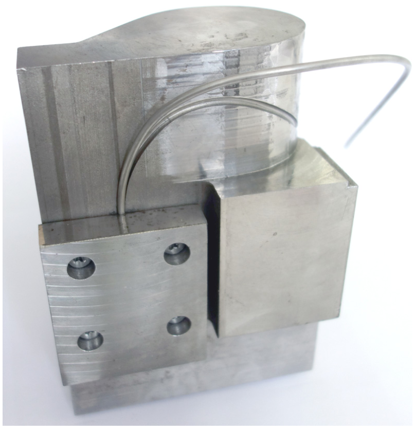
Springback experiment of 3D variable curvature tube bending.

The shape of the tube shown in Figure 11 was measured with the optical measurement system ATOS II 600. The result was an stereolithography (STL) model. This model was compared to the FEM computational model. The two models were registered in one coordinate system. Checking the above results, a maximum difference of 4.76 mm and a minimum difference of −0.76 mm between the computation-ABAQUS and the measurement-STL can be obtained, as shown in Figure 12. The standard deviation is 1.37 mm, and the maximum accuracy deviation is 38.08 mm/m. The results are as shown in Figures 12 and 13, which show that the FEM simulation can effectively predict variable curvature tube-bending springback, while providing the numerical simulation foundation for the establishment of mathematic analytic model for springback prediction of 3D variable curvature tube bending.

Figure 12.

Accuracy deviation of 3D variable curvature tube between FEM and experiment.

Figure 13.

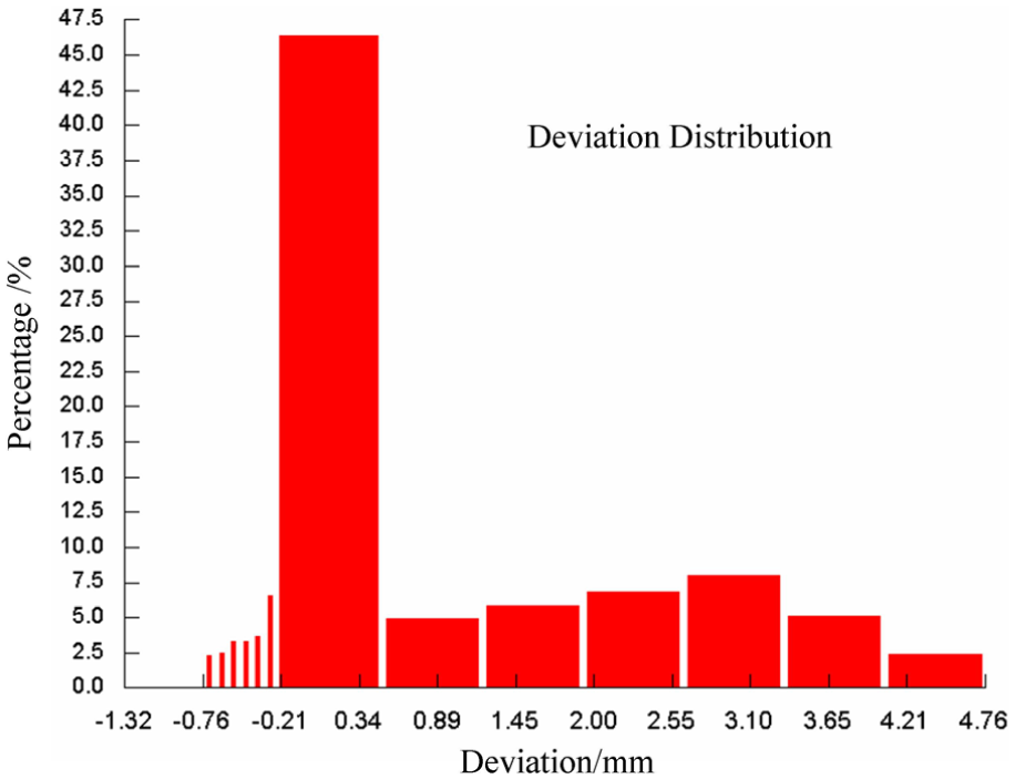
Deviation distribution of 3D variable curvature tube between FEM and experiment.

Mathematic analytic model for springback prediction of 3D variable curvature tube bending

To quickly and accurately predict the springback of 3D variable curvature tube bending, in this article, a mathematic analytic model for springback prediction is established based on the approximate pure bending springback test of tubes. And the direct research of springback problem of variable curvature tube bending in 3D is complex. Then, the 3D springback problem can be transformed into 2D planes in this model.

Springback in three dimensions transformed into two-dimension planes

Partition of 3D variable curvature tube

The axis of 3D variable curvature tube is used as the research object. Due to the complex tube axis, the axis is divided into several sections to simply predict the springback. The curvature of 3D curve expresses the bent degree of curve, and the torsion expresses the torsional degree. To reduce the subsequent arc approximation error, the axis of 3D variable curvature tube is partitioned into a number of sections according to curvature and torsion. As shown in Figure 14, the bent tube axis is partitioned into five parts in a case according to the curvature and torsion.

Figure 14.

Partitioned 3D variable curvature tube axis.

3D tube axis projected onto two planes

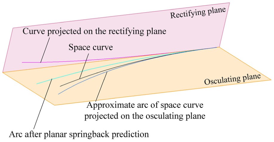
A Frenet frame is established at the initial point of partitioned axis. And the partitioned 3D axis is projected onto base planes named rectifying plane and osculating one.

In this case, the partitioned curves are projected onto rectifying plane and osculating one, keeping the monotonicity on the two planes, as shown in Figure 15.

Figure 15.

Space curve projected onto two base planes.

Springback prediction of 3D variable curvature tube

Springback prediction of partitioned tube

Curve projected on base osculating plane can express curvature changes of space curve projected on the osculating plane. To facilitate springback research and simplify curve geometry expression, the curve projected on the osculating plane is approximated by arcs within 0.15 mm error deviation. The springback problem is researched on the osculating plane by directly using the conclusion of approximate pure bending springback test. The curvature of curve projected on the rectifying plane is small; therefore, the springback will not be used directly. The rectifying planar springback is indirectly considered by jointing corresponding nodes of arc after osculating planar springback prediction and curve projected on the rectifying plane. Through the above means, the discrete planar springback problems can be transformed into 3D.

In this case, the tube-bending radius after springback is calculated by formula (10). The predicted arc of planar springback is obtained by keeping the curves with first-order geometric continuity at the initial point and depending on the principle of arc length changeless, as shown in Figure 16.

Figure 16.

Springback prediction on the osculating plane.

Reverse projection of the new nodes is realized through jointing corresponding nodes of arc after osculating planar springback prediction and curve projected on the rectifying plane. A new non-planar fitting curve is composed by these nodes, by considering the constant length of the curve and the same tangent vector at the initial point, as shown in Figure 17.

Figure 17.

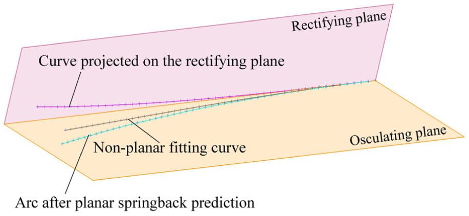
Springback of partitioned non-planar tube axis.

3D joins of partitioned tubes

To predict the springback of the overall 3D tube, the partitioned tubes after springback prediction are jointed in 3D. According to the unchanged factors of curve local Frenet frame, bent tube axis with first-order geometric continuity after springback can be built by coordinate transformation of every curve. Then, the preliminary jointing of partitioned tubes is completed.

Now, take the partitioned tube axes AB and BC as an example, as shown in Figure 18. A Frenet frame is constructed at the endpoint B of curve AB. And a Cartesian coordinate is established taking the principal normal vector as the X-axis, the tangent vector as the Y-axis, and the binormal vector as the Z-axis. In the same way, another Frenet frame and Cartesian coordinate are established at the endpoint of curve 1. Curve 3 is established through coordinate system transformation of curve 2.

Figure 18.

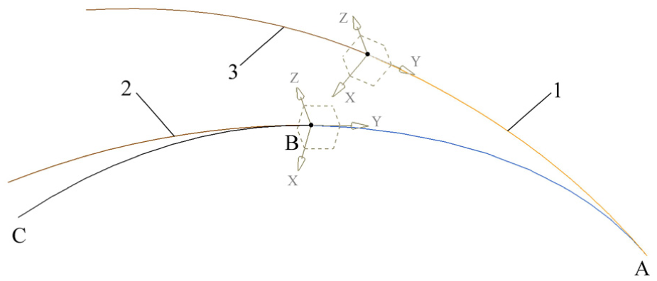
Coordinate transformation of space curve.

Since the tangent vector at the initial point of the partitioned 3D bent tube axes has been corrected. It is mean that the tangent vectors of curves 1 and 3 at the intersection point are in the same direction to ensure the first-order geometric continuity.

Complete coordinate transformation and 3D jointing of partitioned tubes are carried out using the above method. Then, the bent tube axis with first-order geometric continuity after partitioned tube springback prediction is shown in Figure 19.

Figure 19.

Non-planar bent tube axis with first-order geometric continuity after springback.

Correction of partitioned tubes after springback

The final shape of bent tube after springback is the accumulation of the forming process. And the tube-bending process is related to the geometrical shape of the bending die and material characteristics, and so on. The 3D springback problem is more complicated due to the asymmetric stress and deformation and the shear effect caused by the change in curvature. Generally speaking, the greater mutual action of different parts is caused by the more complex tubular shape and the number of bending angles. The superimposed stress will affect the elastic potential energy, which results in reduced springback.

Partitioned tube axes after springback prediction are jointed in three dimensions to get first-order geometric continuity. Springback prediction of each partitioned 3D tube is assumed to approximate pure bending. The springback is the largest in the pure bending state. But in actual conditions, it is difficult to achieve pure bending state. The mutual effect of residual stress in partitioned parts cannot be ignored in the springback process. It is assumed that the effect has been associated with bending complexity, namely, bending curvature and arc length of partitioned tube. A mathematic analytic model, with correction function, for springback prediction of 3D variable curvature tube bending will be established as follows.

The target 3D bent tube axis is divided into a finite number of units. And the axis is recorded as R , constituted by n units. The axis with first-order geometric continuity after the springback of partitioned tubes is recorded as S , so that

$$\mathit{R}=\left\{{\mathit{r}}_i|{\mathit{r}}_i\in R^3,1\le i\le n\right\}$$

(17)

$$\mathit{S}=\left\{{\mathit{s}}_i|{\mathit{s}}_i\in R^3,1\le i\le n\right\}$$

(18)

For node i, ${\mathit{r}}_i$ is transformed to $s_i$ after jointing in the way of first-order geometric continuity. But, actually, the axis after springback is P , which is as follows

$$\mathit{P}=\left\{{\mathit{p}}_i|{\mathit{p}}_i\in R^3,1\le i\le n\right\}$$

(19)

$$\mathit{P}=f(g(A),h(B))=f(\mathit{R},\mathit{S},h(B))$$

(20)

where $g(A)$ is the function related to mechanical performance parameters and boundary conditions of tube bending, which is influenced by R and S . $h(B)$ is the function related to complexity of partitioned tube axes

with

$$w=h(B)$$

(21)

We have

$$\mathit{P}=\mathit{R}+w(\mathit{S}-\mathit{R})\iff {\mathit{p}}_i={\mathit{r}}_i+w({\mathit{s}}_i-{\mathit{r}}_i),\forall i$$

(22)

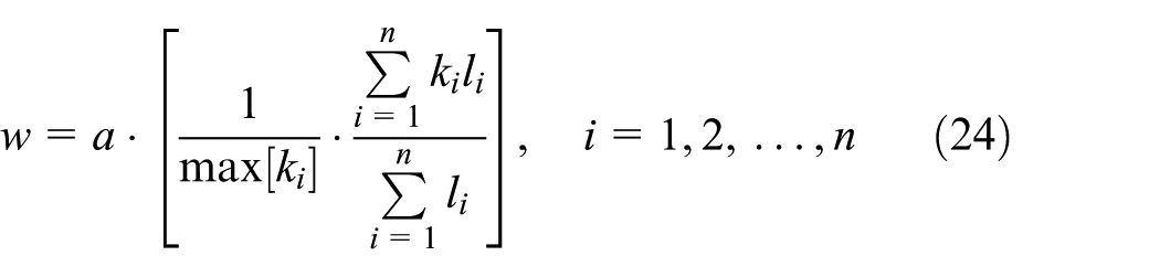
where w is the correction function related to the axis complexity, which is expressed by curvature and torsion. Based on a large number of simulations, we present an empirical equation

$$\begin{array}{cc}\multicolumn{1}{c}{}& w=a·[\frac{1}{\max \left[\sqrt{k_i^2+{\tau }_i^2}\right]}·\frac{\sum _{i=1}^n\sqrt{k_i^2+{\tau }_i^2}{l}_i}{\sum _{i=1}^n{l}_i}],\hfill \\ \multicolumn{1}{c}{}& i=1,2,\dots ,n\hfill \end{array}$$

(23)

where a is the correction factor with the value 1, $k_i$ is the curvature of approximate arc of space curve projected on the osculating plane, ${\tau }_i$ is the torsion at initial point of partitioned non-planar tube axis, and $l_i$ is the axis length of each partitioned tube.

The correction of partitioned tubes after springback can be initially realized by equations (22) and (23). The final bent tube axis is corrected through B-spline fitting according to equal tangent vector at ${\mathit{p}}_1$ and ${\mathit{r}}_1$ . On the above discussion, the mathematic analytic model for springback prediction of 3D variable curvature tube bending is established.

Evaluation of mathematic analytic model for springback prediction

3D tube-bending verification

Example 1

Take the tube-bending model shown in Figure 6 as example. The tube axis after springback can be predicted by the springback prediction analytic model, with w = 0.55 calculated by equation (23), as shown in Figure 20.

Figure 20.

Tube axis after springback using analytic springback prediction model in example 1.

The analytic model and FEM model were registered in one coordinate system. The maximum difference is 3.24 mm and the minimum difference is −0.49 mm between the analytical result and the computation-ABAQUS. The standard deviation is 0.61 mm, and the maximum accuracy deviation is 25.92 mm/m. The results are as shown in Figures 21 and 22. At the same time, the maximum difference is 7.19 mm and the minimum difference is −0.76 mm between the analytical result and the measurement-STL. The standard deviation is 2.17 mm, and the maximum accuracy deviation is 57.52 mm/m. The results are as shown in Figures 23 and 24.

Figure 21.

3D deviation between analytical result and computation-ABAQUS in example 1.

Figure 22.

3D deviation distribution between analytical result and computation-ABAQUS in example 1.

Figure 23.

3D deviation between analytical result and measurement-STL in example 1.

Figure 24.

3D deviation distribution between analytical result and measurement-STL in example 1.

Example 2

In another example, a new bent tube with different material and size is used. The minor-diameter thick-walled tube of high-strength alloy steels with $\varphi$ 3 mm × 0.5 mm (external diameter × wall thickness) and bending length of 161 mm was investigated. The experiment can be finished using the rotary-draw bending die shown in Figure 11. The analytic model with w = 0.55 calculated by equation (23) and measurement-STL model were registered in one coordinate system. The maximum and the minimum difference between them are 4.63 and −0.42 mm, respectively. The standard deviation is 1.28 mm, and the maximum accuracy deviation is 28.76 mm/m. The results are as shown in Figures 25 and 26.

Figure 25.

3D deviation between analytical result and measurement-STL in example 2.

Figure 26.

3D deviation distribution between analytical result and measurement-STL in example 2.

Comparison among FEM simulation, experimental, and analytical results shows good agreements. Maximum accuracy deviation of analytic model is less than 60.00 mm/m (i.e. 6%). The above results show that the mathematic analytic model for springback prediction of 3D variable curvature tube bending is effective.

2D tube-bending verification

In the case of 2D tube bending, the mathematic analytic model discussed above is also applied. ${\tau }_i$ of equation (23) is zero in the case of 2D. So that

$$w=a·[\frac{1}{\max [k_i]}·\frac{\sum _{i=1}^n{k}_i{l}_i}{\sum _{i=1}^n{l}_i}],i=1,2,\dots ,n$$

(24)

Take a 2D minor-diameter thick-walled tube of a steel 0Cr18Ni9 with $\varphi$ 3 mm × 1 mm and bending length of 120 mm for example. The tube axis after springback can be predicted by FEM model and mathematic analytic model with w = 0.67 calculated by equation (24). The experiment can be finished using the rotary-draw bending die shown in the Figure 27. The analytic model, FEM model, and measurement-STL were registered in one coordinate system. The maximum difference is 2.48 mm and the average difference is 0.52 mm between the analytical result and the computation-ABAQUS. The maximum accuracy deviation is 20.67 mm/m, and the average accuracy deviation is 4.33 mm/m. At the same time, the maximum difference is 3.70 mm and the average one is 0.78 mm between the analytical result and the measurement-STL. The maximum accuracy deviation is 30.83 mm/m and the average one is 6.50 mm/m. The results are as shown in Figures 28 and 29.

Figure 27.

Springback experiment of 2D variable curvature tube bending.

Figure 28.

Springback axis of 2D variable curvature tube bending.

Figure 29.

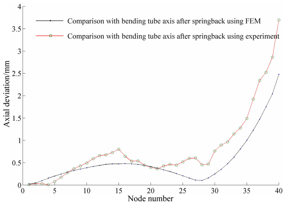
Axial deviation of 2D variable curvature tube bending.

Comparison among FEM simulation, experimental, and analytical results shows good agreements. The maximum accuracy deviation of the analytic model is less than 50.00 mm/m (i.e. 5%). The above results show that the mathematic analytic model for springback prediction can also be applied to the 2D condition.

Errors analysis

Springback prediction error sources of analytic model can be mainly summed up from the following three aspects:

1. Error caused by torsion springback. Torsion springback is a common phenomenon in 3D variable curvature tube-bending process. This article directly predicts the tube axis projected on the osculating plane to simplify springback prediction, while the torsion springback is not considered particularly.

2. Error of data fitting caused by approximate pure bending springback test. The least squares method is used for the polynomial fitting of experiment data, which causes error accumulation for springback prediction.

3. Arc approximate error. Arc approximate of plane curve for the springback prediction on the projection plane causes error accumulation. In this article, the approximate error is less than 0.15 mm.

Conclusion

In this article, based on the tube-bending springback properties, new FE simulation method, analytic calculation method, and experiment method have been built. The main purpose of such methods is to reveal the bending mechanism and to solve the immatureness problem of variable curvature (variable curvature of the plane and space) tube bending. The study in this article resolves the springback control of variable curvature bending problem for minor-diameter thick-walled tube, which can provide significant benefit to accurate forming of the variable curvature bended tube.