
Abstract
In order to study the spatial breakup characteristics of the initial section of low-pressure jets, an experiment was performed to investigate the flow fields and concentration fields of jet flows with different nozzle geometric parameters and also the different working pressures using a particle image velocimetry system. The flow field of different axial planes, axial time-average velocity, and the length of the initial sections of jet flows were also analyzed. A numerical simulation was carried out using finite volume method and volume of fluid–level set method to describe the breaking process of the initial section, capturing unstable development of gas–fluid interface, measuring the length of the initial sections of jet flows. Both experiment and simulation results show that the broken degree of jet is more intense for nozzles with smaller aspect ratio; the outlet velocity of jet increases with the working pressure; and the value of
Keywords
Introduction
The free surface flow of low-pressure jet and gas–liquid interface flow has attracted many researches in agricultural sprinkling irrigation for the purpose of uniform spraying. The interaction between liquid jet and air is complex in two-phase flow, and the breakup property of fluid flow field will directly affect the spraying uniformity.1,2 For the key fluidic element, the circular nozzle, there are many studies that reported the effect of nozzle geometric parameters on jet external characteristics than the effect of spatial breakup property. With the development of laser measuring technology, flow visualization technology,3–6 and computational fluid dynamics (CFD) software,7,8 the jet flow rules in air can be better studied.
At present, noninvasive measuring techniques have been proposed to describe the flow properties through computational visualization methodologies such as particle image velocimetry (PIV), particle tracking velocimetry (PTV), and phase Doppler particle anemometry (PDPA) for two-dimensional flow analysis. Those techniques were mainly used for the measuring of atomization jets, in which the nozzle has a small bore or working under the high pressure and temperature. Techniques, such as phase Doppler anemometry (PDA) were employed to characterize the Sauter mean diameter (SMD) and velocity vectors of the starch–urea–borax. 9 Digital particle image velocimetry (DPIV) technique was used to measure the turbulent flow of cylindrical jet with different Reynolds numbers at outlets, 10 and the distribution of average vorticity and instantaneous vorticity in jet development area was obtained. The effect of outlet geometric parameters of cross-flow on flow characteristics in the near field was researched by PIV. 11 The characteristics of time averaged and turbulent flow in the jet mixing process were researched with PIV and laser-induced fluorescence (LIF). 12 The detailed droplet motion distribution of swirling nozzle was studied and obtained by PIV. 13 PDPA was applied to measure nonintrusively typical parameters such as average velocity, root mean square (RMS) velocity, and droplet diameter of a fan water jet flow. 14
For the numerical simulation studies of atomization jet, the physical process of the initial atomization in high-pressure jet was simulated using the direct numerical simulation (DNS) model, and the link near the nozzle and the dynamic performances of droplets were selectively analyzed. 15 Simulations of the capillary instability process and the breakup of a jet were carried out using a one-fluid model to describe the two-phase flow and a volume of fluid (VOF) approach to capture the interface. 16 A simple VOF coupled with level set (LS) method (S-CLSVOF) for improving surface tension was proposed and tested compared to a standard VOF solver and experimental observations.17,18 A three-dimensional (3D) code was developed, 19 where interface tracking was performed by a LS method, and the ghost fluid method was used to capture sharp discontinuities accurately; the LS and VOF methods were coupled to ensure mass conservation. 20 Arnaud et al. 21 did a simulation of the jet breakup in biphasic conditions; results reveal that in the range of investigated Reynolds and Ohnesorge numbers, the classical criteria used to distinguish the different modes of jet breakup at atmospheric pressure seems to be valid for the high-pressure environment. The jet atomization was numerically simulated with high We number and Re number, with analyses on the initial breakup process and comparison among the different atomization states under two jet models. 22 The relationship between jet core length and We number was explored, and the characteristics of the distribution of velocity field and pressure field were analyzed. 23
Above all, previous studies mainly focused on atomization jets with small-bore nozzle under high pressures or large-caliber nozzle under low pressures and high temperature for the chemical and fuel injection, while few researches were carried out on jets with large-caliber nozzle under low pressures for the sprinkling irrigation, in which the jet has a long jet breakup length. Therefore, this article reports the characterization of jet breakup by changing the structural parameters and working pressure of nozzle, with the application of PIV technology and numerical simulation method. The specific goals of this study are as follows: (1) to obtain the flow field of different axial planes, vortex field, time-average velocity distribution, and the length of core section of jet flows using PIV; and (2) to compare the experimental data with simulation results, for validating the accuracy and reliability of the PIV experiment and the CFD simulation, which will lay the foundation of spatial jet breakup characteristic research.
Materials and methods
Experimental setup
The experimental setup is schematically presented in Figure 1, which is composed of two parts: the jet system and the PIV system. The jet system was composed of (1) a water tank with a capacity of 1 m3; (2) a centrifugal pump with a power of 5.5 kW and pipes equipped with valves, a lateral flowmeter, and a 600-kPa ABS radial manometer manufactured by Fimet; (3) a rocker-type sprinkler manufactured by WadeRain, type PY115, with a nozzle angle of 23° with respect to the horizontal; and (4) 20-mm-diameter SUS pipes.
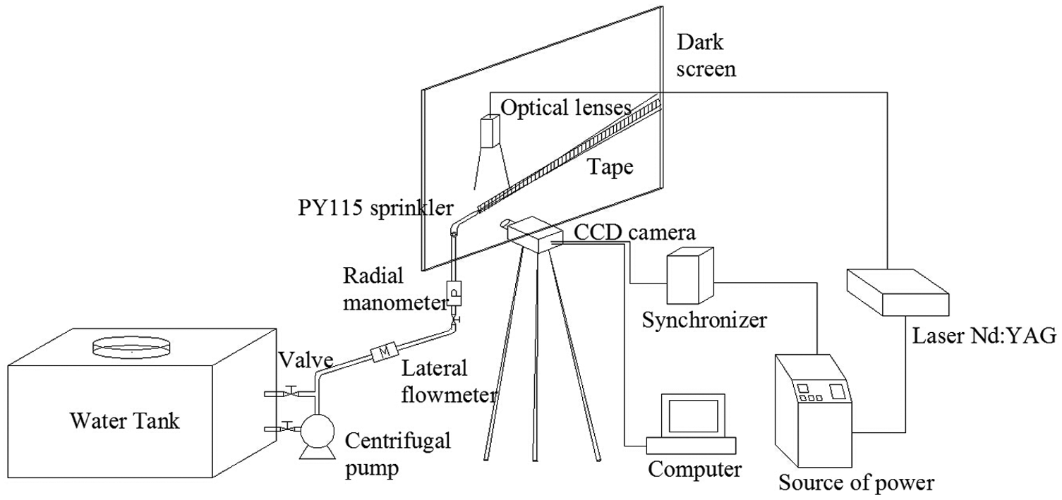
Experimental setup for jet flow characteristic observation using PIV.
The PIV system used in this research was composed of three subsystems: (1) an imaging system composed of pulsed laser, guiding beam arm, a set of optical accessories (mirrors and lenses), and image acquisition system. Among them, the pulsed laser beam was generated by a Nd:YAG laser with a power of 200 mJ. The frame straddling charge-coupled device (CCD; PowerView™ Plus 4MP model) was used, with a temporal resolution of 60 frames/s and a spatial resolution of 640 × 480 pixels; (2) an analysis display system composed of INSIGHT 3G software for image processing, embedded with TECPLOT and MATLAB; and (3) a synchronous control system composed of the synchronizer (trigger) type 610035 to control the image acquisition sequence and the laser light triggering.
Selection of nozzle models
The PY115 sprinkler was selected as a prototype in this article, as presented in Figure 2. Figure 3 presents the nozzle with different geometric parameters including the jet orifice diameter

Prototype sprinkler of PY115.

Structure of the nozzle.
Parameters of five nozzle types.

PIV experimental principle and procedure
The experiment was carried out using the PIV visualization technology to observe the jet flow field. PIV technique is realized based on recording the scattered light information of the two particle swarms with short intervals and then processed the relevant data of the two images and finally obtained the velocity field. For evaluation of an average displacement, the images were divided into small subareas called “interrogation windows” (typically 128 × 128, down to 16 × 16 pixels). The local displacement vector for the images was then determined for each interrogation window by means of cross-correlation as illustrated in Figure 4. Essentially, the cross-correlation function statistically measures the degree of match between the two samples. The location of the highest correlation peak in the correlation plane can then be used as a direct measure of the average particle displacement. The vector of the local flow velocity (in the plane of the light sheet) was calculated, taking into account the time delay between the two images and the magnification factor of the image. INSIGHT 3G software was used to process the data, and the velocity fields were tested, as shown later in the “Results and discussion” section.

Principle of PIV measurements, using cross-correlation between two successive frames.
Post-processing involves data validation, removal of erroneous data, replacement of removed data, and data smoothing or optimization. Raw images will always suffer from noise form, reflections, or low seeding density. Random noise is normally not a problem, as it does not severely affect the correlation function. Flow images, however, are not always perfectly random, and periodic patterns correlate well and will modify the correlation function, which can lead to erroneous vectors. A criterion used to eliminate unreliable vectors is the ratio of the largest to the second largest peak in the cross-correlation. In this study, the maximum value of jet velocity was used as a criterion.
The experimental site provides the environment to carry out hydraulic performance tests of the sprinkler under windless conditions, and the flow rate and the working pressure were controlled by valve. In this article, the pressure was the main consideration, which was supplied by a power pack. It had an integrated water tank, with water continuously being flushed through the tank to keep a constant water temperature. The pump is a centrifugal pump, which can give variations in the pressure. The working pressure was in the range of 200–400 kPa, and the values were measured using a manometer with an accuracy of 0.4.
The glass microsphere was used as seeding particles with 1 µm diameter, which was added to the water tank and mixed with water. The valve was kept opened, and the working pressure required in the experiment was adjusted. To better capture the PIV images, optical lenses were placed on the top of jet, and the laser penetrated the jet from top to bottom. The removable dark screen and CCD camera were positioned vertically at the two sides of jet; the tape was stuck on the dark screen parallel to the track of injection flow, which was used to adjust the horizontal moving distance of dark screen and CCD camera by referring to its scale. The horizontal distance between CCD camera and jet flow could be adjusted due to the limit of scattering area of laser, as shown in Figure 5.

Diagram of the jet flow characteristics.
Numerical simulation
An investigation of the breakup characteristics such as the initial length of jet was performed by evaluating the pressure and the geometric parameters of the nozzle. The measurements were performed, and the pressure was varied from 200 to 400 kPa with nozzle type varied from A to E. A two-phase model was adopted to describe the breakup characteristics of low-pressure jet in spatial flow field which is subjected to the gas–liquid interaction.
ANSYS ICEM software was used to create the geometry and meshing as shown in Figure 6. Meanwhile, the grid independence was evaluated by adopting four grid sizes for the computational domain at a pressure of 400 kPa with nozzle type B, the results are shown in Table 2. Grid 2 represents the grid independence because the difference in breakup length between the second and the fourth grids was <0.7%.

3D view of the simulation sections.
Grid independence analysis results for type B nozzle when p = 400 kPa.

The governing equations were solved by CFD software ANSYS FLUENT 14.0 based on the associated boundary and initial conditions. The finite volume method was applied to discretize the governing equations in the computational domain. The renormalization group (RNG)
Governing equations
At present, there are two main ways to solve the interface problem of the interaction between the two liquids: the LS method and the VOF method, and both are Euler methods. The LS method is suitable to solve the problem of interface curvature; the VOF method is simpler, and it can maintain the conservation of fluid volume in calculation. VOF method can avoid the nonconservation of mass which exists in LS method; besides, the solution of normal direction and precision of curvature can be optimized using LS method. Therefore, the basic idea of CLSVOF which contains two methods was recently proposed by some scholars. This article will research the spatial breakup characteristics of the core section of low-pressure jet using the CLSVOF method.
The continuity equation, momentum equation, and energy equation have been used to serve as a control equation to solve problems in gas–liquid two-phase flow process. Without considering the influence of temperature to the flow, the control equation of single phase and mixed phase of two-phase flow was written in a uniform form, as follows

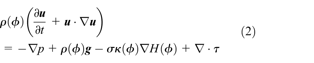

where
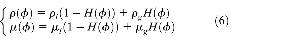
The form of Heaviside function could be expressed as

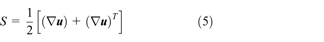
where h is the mesh size. The mathematics of strain rate tensor (
The value of different areas of
Results and discussion
Measurement of velocity field in jet flows
Figure 7 shows the particle image and the velocity field of jet flow with type B nozzle under different pressures. Figure 8 shows the particle image and the velocity field of jet flow with different nozzle types at a pressure of 400 kPa. The normalization is used in coordinates in this figure; the coordinate scale is
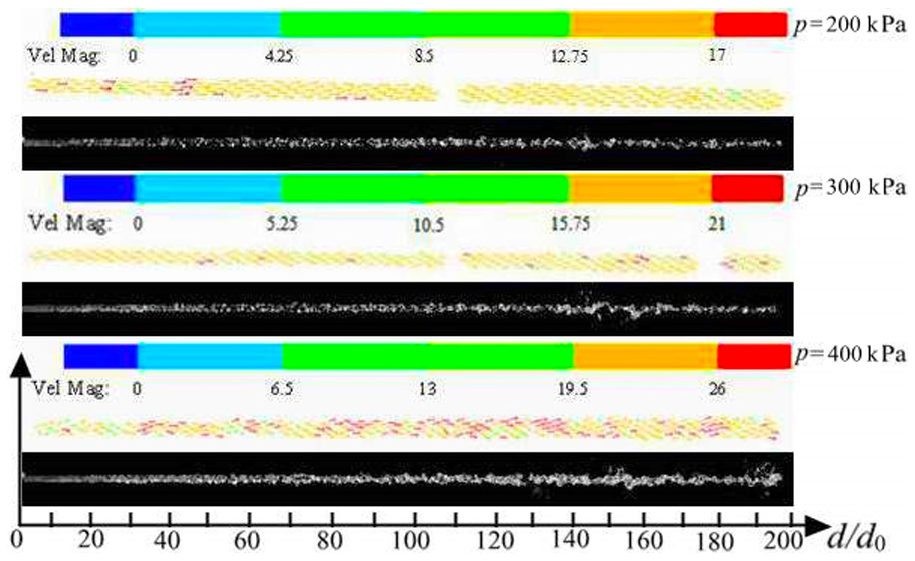
Velocity field of jet flows under different pressures (type B nozzle).

Velocity field of jet flows with different nozzle types (400 kPa).
As shown in Figure 7, the jet flow shoot into the air with the turbulence flow pattern. The boundary line of jet flow is not a smooth straight line but a zigzag line. With an increase in pressure, the breakup degree of the jet becomes severe. The velocity fields are significantly different under different working pressures, and the outlet velocity of jet flow increases with the increasing pressures, and the breakup length of jet becomes longer with the increasing pressures. Figure 7 also shows that the breakup section of the jet occurs when there is no velocity. Because of the breaking of jets, the movement of the tracer particles was not captured by the laser, and the velocity could not be extracted.
In Figure 8, under different nozzle type conditions, the jet presents different patterns. The jet breakup degree with type C and type E nozzles are violent, and the lengths of the breakup section are shorter, which means that the jet broken degree is more intense with smaller aspect ratio. The velocity field of jet flows is different for different nozzle types. The turbulence intensity is different because of the difference in the nozzle parameters, resulting from the different velocity field distributions. Comparing the five nozzles at the same pressure, the outlet velocity of jet flows with type A and type D nozzles are the largest, while it is lower with type C and type E nozzles. The distribution width of velocity field with type E nozzle is the widest, which means the jet has been seriously affected by the air.
Measurement of the initial lengths
Free jet is composed of the initial section, the transition section, and the breakup section. A ratio of
Figure 9 shows the time-average velocity distribution of jet flows along the axial direction with different pressures and nozzle types. The variation ranges and average values of

Flow velocity distribution of jet flows along the axial direction: (a) type B nozzle with different pressures and (b) different nozzle types at a pressure of 400 kPa.
Fluid-phase nephogram and velocity distribution
Contours of liquid volume fraction of the jet are illustrated in Figure 10 using the sprinkler with type B nozzle under three different pressures. The lengths of the jet breakup section were analyzed with the ScanIt software, which shows that it increases with the working pressure, and the magnitudes are 510.1, 606.8, and 642.4 mm. The results indicated that the range of jet could be larger with an increasing pressure.

Contours of liquid volume fraction with type B nozzle under different pressures: (a) 200 kPa, (b) 300 kPa, and (c) 400 kPa.
Figure 11 presents the velocity distribution of jet flows under different pressures. In this figure, the outlet velocity of jet increases with the increasing working pressures, and the velocity along the jet axial direction decreases when the range increases. With the entrainment of air into the jets, the amount of fluid which moves with jet continuously increases, and the jet boundary extends to the sides with, besides, the increased flow friction. Due to the principle of the mixture of jet and static flow, the resistance of the jet will be larger, and the velocity on the edge of jet will decrease.

Contours of velocity magnitude with type B nozzle under different pressures: (a) 200 kPa, (b) 300 kPa, and (c) 400 kPa.
Flow velocity distribution along the radial direction of jet flows
In Figure 12,

Flow velocity distribution in the cross section of jet flows with type B nozzle: (a)
Figure 12(a) shows that the flow velocity distribution in the cross section of jet flow with type B nozzle at the pressure of 200 kPa basically agrees well with Gauss normal distribution, which shows that the jet flow has reached the fully developed turbulent flow with
Comparison between PIV experiment and numerical simulation
Figure 13 shows the comparison between the experimental velocity of jet and the numerical simulation for the sprinkler with type B nozzle under different pressures. It shows that for the five pressures, the trend of simulation values is the same as experimental values. At the same point of cross section, experimental values of velocity are slightly higher than the simulation values. However, there is a good agreement between numerical and experimental data with an error of <8%, which means that there are different pressure fluctuations of jet in the experiment, leading to an increase in the flow velocity. Differently, the simulation is just considered as an ideal state without any outside influence on the jet.

Comparison of flow velocity distribution in the cross section of jet flows with
The numerical results for the tested
Length of the initial sections of jet flows with different pressures and nozzle types.

E. V: experimental value; S.V: simulation value.
Conclusion
This article presents the advanced applications of PIV technique and numerical simulation method to measure the flow field of different axial planes, axial time-average velocity, and the length of the initial sections of jet flows emitted by the sprinkler with different nozzle geometric parameters and working pressures. From the results of this study, the following conclusions can be drawn:
In the experimental conditions, for the same type nozzle, the outlet velocity of jet flow increases with an increase in pressure which resulted in the initial length of jet becoming longer. Comparing five nozzles having different aspect ratios with the same pressure showed a broken degree of jet. It was more intense with the smaller aspect ratio, and the outlet velocity of jet flow with larger aspect ratio was the largest. The length of the initial section with larger aspect ratio is the longest and which is the shortest with the small aspect ratio.
In the numerical simulation conditions, for the same type nozzle, the initial length of jet also increases with the increase in the working pressures. In the same cross section of jet, the value of
Information provided in this article can lead to the refinement of the PIV technique and numerical simulation method for their applications to sprinklers. Further research should concentrate on the comparisons between experiment and numerical simulation about the further breakup and coalescence of the droplets formed after the primary atomization and on the analysis of wind effects on jet flow. In this case, the models in further study on the research of atomization mechanism will be improved.
Footnotes
Academic Editor: Nao-Aki Noda
Declaration of conflicting interests
The author(s) declared no potential conflicts of interest with respect to the research, authorship, and/or publication of this article.
Funding
The author(s) disclosed receipt of the following financial support for the research, authorship, and/or publication of this article: We are grateful for the financial support from the National Natural Science Foundation of China (no. 51279068 and 51379090), Special Fund for Ago-scientific Research in the Public Interest of China (no. 201503130), Jiangsu Scientific Research and Innovation Program for Graduates in the Universities (no. KYLX_1041), and the Project Funded by the Priority Academic Program Development of Jiangsu Higher Education Institutions (PAPD).