Development of a hybrid multi-scale simulation approach for spray processes

Abstract

This paper presents a multi-scale approach coupling a Eulerian interface-tracking method and a Lagrangian particle-tracking method to simulate liquid atomisation processes. This method aims to represent the complete spray atomisation process including the primary break-up process and the secondary break-up process, paving the way for high-fidelity simulations of spray atomisation in the dense spray zone and spray combustion in the dilute spray zone. The Eulerian method is based on the coupled level-set and volume-of-fluid method for interface tracking, which can accurately simulate the primary break-up process. For the coupling approach, the Eulerian method describes only large droplet and ligament structures, while small-scale droplet structures are removed from the resolved Eulerian description and transformed into Lagrangian point-source spherical droplets. The Lagrangian method is thus used to track smaller droplets. In this study, two-dimensional simulations of liquid jet atomisation are performed. We analysed Lagrangian droplet formation and motion using the multi-scale approach. The results indicate that the coupling method successfully achieves multi-scale simulations and accurately models droplet motion after the Eulerian–Lagrangian transition. Finally, the reverse Lagrangian–Eulerian transition is also considered to cope with interactions between Eulerian droplets and Lagrangian droplets.

Keywords

Multi-scale approach coupled level-set and volume-of-fluid method point particle spray atomisation

Introduction

Energy conversion in transportation is usually related to the transfer of chemical energy to sensible energy, which is widely achieved by spray combustion. For instance, liquid fuel injection is one of the most common procedures in non-premixed combustion systems such as internal-combustion engines and aircraft gas turbine combustors for road and air transportation. It plays a significant role in achieving an efficient and clean combustion process. A large number of studies have been devoted to better understanding of the atomisation process.^1–6 The main aim is to understand accurately the physiochemical spray process and to predict the two-phase multi-scale flow characteristics and the subsequent combustion process. However, detailed local quantitative information such as the liquid–gas interface formation and the break-up mechanisms are not well understood yet. Thus, there is an urgent need to improve the understanding of the spray flow characteristics, especially the primary break-up and the secondary break-up in both the dense spray regime and the dilute spray regime, using an efficient computational method.

Spray atomisation is a complex process, which can be divided into three regimes.^{2, 7} The first is the liquid core zone in which the liquid area is very dense and appears as a continuum fluid; the second is the dispersed flow zone in which the liquid can be approximated as dispersed particles; the last is the transition zone. There are a variety of numerical methods today that can be used to examine this spray atomisation process. However, it is noted that a large class of applications uses only a pure Lagrangian method for areas far away from the nozzle in the dilute spray regime⁸ or only a pure Eulerian approach for areas near the nozzle^{9, 10} in the dense spray regime.

In order to simulate accurately and efficiently the spray process including the different zones, efforts have been made in recent years and some multi-scale methods have been proposed, such as Eulerian–Lagrangian spray atomisation (ELSA),¹¹ the combined coupled level-set and volume-of-fluid (CLSVOF) method (or the volume-of-fluid (VOF) method) and the Lagrangian particle-tracking method.^12–15 The ELSA method proposed by Vallet et al.¹⁶ is to predict realistically the dilute zone and the dense zone of a spray atomisation process. In this method, the gas phase and the liquid phase are considered as species, and a liquid–gas surface density function is used to describe the interface area. With rapidly growing computational resources and development of numerical approaches, more accurate Eulerian methods such as the VOF method, the level-set method¹⁷ and the CLSVOF method¹⁸ have been used to explore the complex behaviour of dispersed multi-phase flows.¹⁹ In these methods, the interface-tracking algorithms can accurately represent the liquid–gas interfaces, their positions and their geometries. However, when thin ligaments form and subsequently break up into droplets, especially in the dilute regime, small droplets require much finer grid resolutions, which greatly increase the computational cost.¹⁵ Thus, a coupling method is employed to deal with the small droplets using a Lagrangian method with lower grid resolution requirement while retaining the advantage of the Eulerian method to track the liquid–gas interfaces accurately. The advantage of this coupled method is to achieve sufficient computational accuracy on different scales including the dense spray regime and the dilute spray regime. Through the multi-grid strategy such as adaptive mesh refinement²⁰ and a refined level-set grid,²¹ the coupled method has a great potential to reduce the computational cost effectively in the dilute regime and to achieve simulations of a real-scale spray in industrial applications.

In the multi-scale coupling method, a Eulerian method is used to track or represent liquid–gas interfaces in the primary break-up regime (the liquid core zone), and a Lagrangian droplet tracking method is used to trace the dispersed small droplets in the dilute spray zone. The coupling procedure between the two methods is currently under active development and also the focus of this paper. Proposing a hybrid method for multi-scale two-phase flow is challenging. Our main contribution of this paper is to demonstrate the achievement of the transformation of small droplets in detail from a Eulerian structure to a Lagrangian particle and the reverse transition process, and the performance of the coupled method based on the combination of the CLSVOF (Eulerian) method and the KIVA (Lagrangian) method in simulating a liquid jet process.

As an outline of the paper, the numerical models including the CLSVOF model, the Lagrangian particle-tracking method and the coupling approach will be presented in the second section. The third section introduces the computational set-up. In the fourth section, we present the results and a discussion. Conclusions are given in the fifth section.

Numerical methods

The CLSVOF method

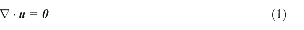
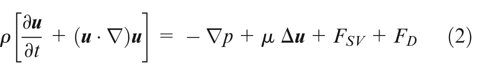
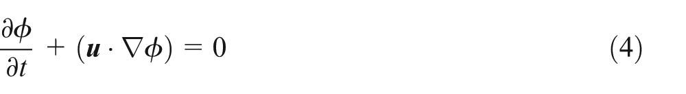
A CLSVOF method³ is used here to represent and obtain the evolution of liquid–gas interfaces. The governing equations to be solved are

\nabla \cdot u = 0

(1)

ρ [\frac{\partial u}{\partial t} + (u \cdot \nabla) u] = - \nabla p + μ Δ u + F_{SV} + F_{D}

(2)

where u is the velocity vector, ρ is the density, p is the pressure and μ is the viscosity. Both the liquid phase and the gas phase are Newtonian fluids. The pressure is obtained by solving the Poisson equation iteratively. F_D represents the effect of the dispersed phase simulated using the Lagrangian approach on the flow according to

F_{D} = \sum_{i = 0}^{n_{d}} \frac{4}{3} π ρ_{l} r_{d} (v_{d, i}^{n + 1} - v_{d, i}^{n})

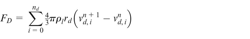
where n_d is the total number of Lagrangian droplets in one cell, ρ_l is the density of liquid droplets and r_d is the radius of liquid droplets.

F_SV is the surface tension term and is calculated by the continuum surface force method²² as

F_{SV} = σ κ \frac{\nabla ϕ}{ϕ_{\max} - ϕ_{\min}}

(3)

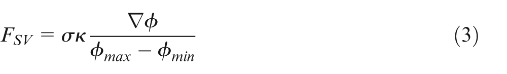
where σ is the surface tension coefficient, κ is the local curvature and ϕ is the colour function with ϕ = 0 for gas and ϕ = 1 for liquid. The colour function ϕ can be expressed as

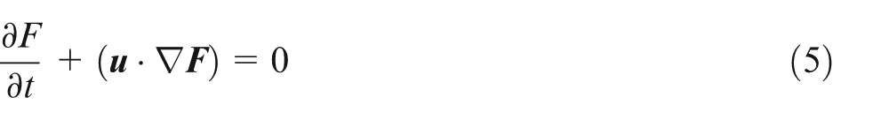
\frac{\partial ϕ}{\partial t} + (u \cdot \nabla ϕ) = 0

(4)

For our work, liquid–gas interfaces are obtained by the level-set method. In the level-set method, the function F (a signed distance function) is solved instead of directly solving ϕ. A liquid–gas interface is defined as F = 0. Thus the equation for F can be written as

\frac{\partial F}{\partial t} + (u \cdot \nabla F) = 0

(5)

To improve the volume conservation, a modified VOF method called the multi-interface advection and reconstruction solver is incorporated.

On the assumptions that ρ and μ are constant within each fluid, they can be calculated from

ρ = H (F) ρ_{l} + [1 - H (F)] ρ_{g}

(6)

μ = H (F) μ_{l} + [1 - H (F)] μ_{g}

(7)

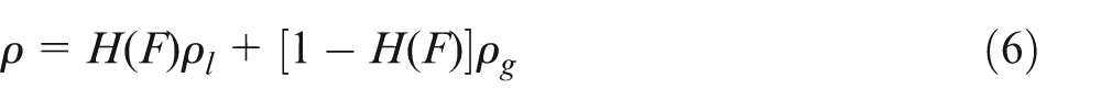
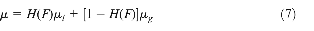
where the subscripts l and g denote liquid and gas respectively and $H$ is the Heaviside function.

Lagrangian particle tracking method

The Lagrangian method is based on a modified version of KIVA-3V.^{23, 24} In the Lagrangian method, the droplet velocity is determined by the drag force F_i ,_d on the droplet, which is in turn determined by the relative velocity between the liquid droplet and the gas phase. The droplet velocity equation is²³

\begin{matrix} \frac{d v_{d, i}}{d t} & = \frac{F_{i, d}}{m_{d}} \\ = \frac{0.375 (ρ / ρ_{l}) | V_{vel} |}{r_{d} V_{vel} C_{D}} \end{matrix}

(8)

where $m_{d} = \frac{4}{3} π ρ_{l} r_{d}^{3}$ is the droplet mass, V_vel is the relative velocity between the liquid drop and the gas and C_D,sphere is the drop drag coefficient given by

C_{D} = {\begin{matrix} \frac{24}{{Re}_{d}} (1 + \frac{1}{6} {Re}_{d}^{2 / 3}), {Re}_{d} \leq 1000 \\ 0.424, {Re}_{d} > 1000 \end{matrix}

(9)

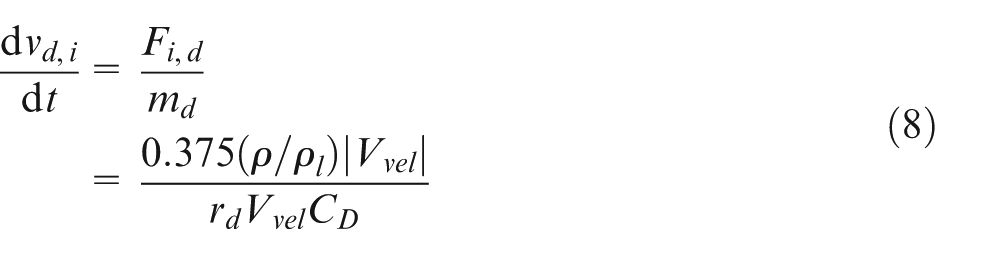
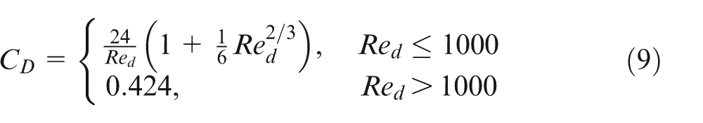
where Re_d is the droplet Reynolds number.

The relative velocity V_vel is $V_{vel} = {\tilde{u}}_{i} - v_{d, i}$ and is calculated using the gas velocity at the droplet position ${\tilde{u}}_{i}$ , which is obtained in the Eulerian framework, and the droplet velocity v_d ,_i. The interpolation scheme proposed by Nordin²⁵ is utilised, which considered eight vertices of the cell at the droplet location and used an inverse distance weighting method. Considering the effect of droplet deformation in shape, the above drag coefficient is revised by a drop distortion coefficient²⁶ y_p . Thus the final equation for C_D is C_D = C_D,sphere (1 + 2.632y_p ). In the limits of no distortion (y_p = 0) and maximum distortion (y_p = 1), the rigid sphere coefficient and the disc drag coefficient are recovered respectively.

Eulerian–Lagrangian droplet transition

In this section, the droplet transition from a Eulerian structure to a Lagrangian particle is detailed, which is divided into three steps.¹²

First, isolated droplets need to be identified and their mass, velocity and temperature are determined. In our work, we use a neighbour-searching algorithm to identify an isolated liquid structure. In order to achieve this process, we set a G function which is similar to the colour function ϕ with ϕ = 0 for gas and ϕ = 1 for liquid used in the level-set method. Initially, G = ϕ. Thus, G = 1 represents liquid, and G = 0 is the gas field. At every time step, we tag all isolated liquid structures. (First, when a cell with G = 1 is identified, the value G of the cell is tagged G = 2 and at the same time a start is made to search its neighbouring cells (including two directions for a two-dimensional case); if G = 1 is found, the neighbouring cell will also be set to G = 2 and added to the same list. Eventually, all the neighbouring cells of this list all have G = 0 or G = 2; then, the isolated droplet structure is identified. Next, we start to search for the next cell with G = 1 and set G = 3. Following this procedure, all isolated droplet structures can be identified.) It is important to note that only the G = 1 cells need to be searched for in our program to reduce the computational cost.

Second, we set up the conversion criteria for the Eulerian–Lagrangian transition. Whether or not a Eulerian structure will be transformed into a Lagrangian particle is determined by the critical volume of the Eulerian structure and the critical length of the thin isolated ligament identified. In this work, we use two different grids: one for the CLSVOF method and the other for the KIVA method. The critical volume is set to be the KIVA cell volume. Therefore, the first conversion criterion is V_Eulerian < 0.5V_KIVAgrid , where V_Eulerian and V_KIVAgrid are the Eulerian droplet volume and the KIVA grid cell volume respectively. 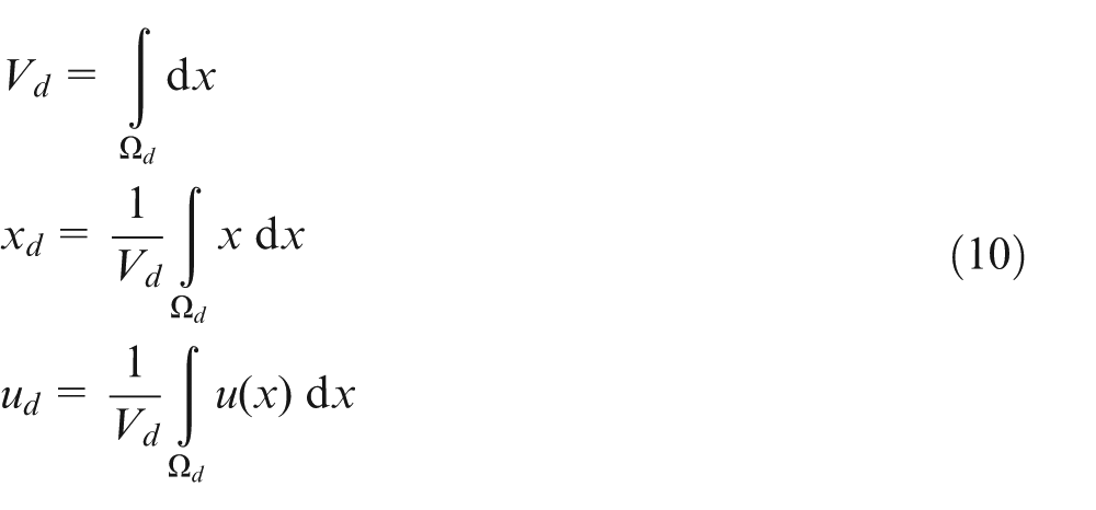In order to calculate accurately the further break-up process of a largely deformed thin ligament in the Eulerian description despite the fact that the Eulerian droplet volume meets the first criterion, the second criterion is $α \geq R_{\max} / \max {Δ x, {[(3 / 4 π) V_{Eulerian}]}^{1 / 3}}$ , where R_max is the maximum distance from the edge of a Eulerian droplet to the centre of mass of the Eulerian droplet. In this paper the criterion parameter α is equal to 4.

Third, isolated droplets that meet the conversion criteria from the Eulerian description are removed. At the same time, the removed droplets are transformed to Lagrangian particles with a determined droplet mass and velocity. To accomplish this removal process, some terms need to be revised, including the volume fraction function ϕ (ϕ = 0) and the distance function $F (F = | F |)$ .

While this operation is completed, the droplet volume V_d , the centre x_d of mass and the velocity u_d are calculated as

\begin{matrix} V_{d} = \int_{Ω_{d}} d x \\ x_{d} = \frac{1}{V_{d}} \int_{Ω_{d}} x d x \\ u_{d} = \frac{1}{V_{d}} \int_{Ω_{d}} u (x) d x \end{matrix}

(10)

Lagrangian–Eulerian droplet transition

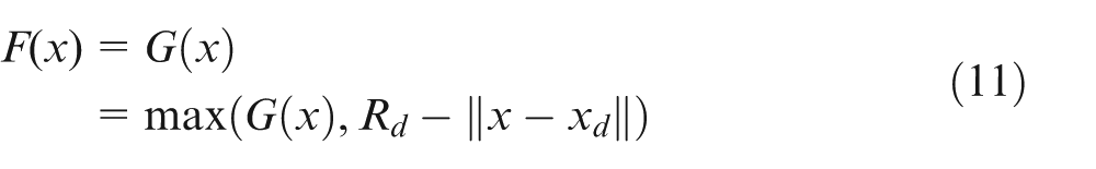
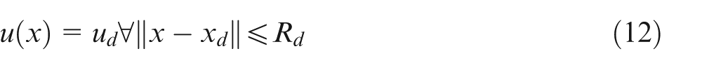
The previous section introduces the transition process from a Eulerian droplet structure to a Lagrangian particle. A reverse transition will be needed when a Lagrangian particle collides with a Eulerian structure. In the present study, first, if the distance G(x_d ) of the centre of a Lagrangian droplet to the surface of a Eulerian structure is less than the Lagrangian droplet radius (i.e. G(x_d ) < R_d ) and, second, if the size of the Lagrangian droplet is larger than the local 2 × 2 Eulerian grids, the transition process occurs.

Once the reverse transition occurs, the droplet volume V_d and the centre x_d of mass can be easily calculated according to the above method. The level-set function needs to be re-evaluated in a certain area (extended by six cells in each direction from the local liquid–gas interface)¹⁴ according to

\begin{matrix} F (x) & = G (x) \\ = \max (G (x), R_{d} - ‖ x - x_{d} ‖) \end{matrix}

(11)

The VOF function ϕ is recalculated using the level-set function.

The transition of the droplet momentum is a more challenging task. In this paper, we simply set the Eulerian droplet velocity to be equal to the Lagrangian point-particle velocity according to the solid-sphere assumption, as given by

u (x) = u_{d} \forall ‖ x - x_{d} ‖ \leq R_{d}

(12)

Finally, it should be stressed that, since the CLSVOF method cannot support very small droplets whose sizes are below a certain magnitude, not all the Lagrangian droplets are transferred back to Eulerian droplets when they are interacting with a Eulerian structure. In the present study, the threshold is set to be V _2 × 2E; thus, it is only if the size of a Lagrangian droplet is larger than the local 2 × 2 Eulerian grids (the second condition as stated above) that the transition is performed. Otherwise, the Lagrangian droplet is maintained as a point particle, and its interaction with Eulerian structures is approximated.

Case set-up

In this paper, liquid jet injection into quiescent high-pressure air is considered. The nozzle diameter D is 0.08 mm and the injection velocity is 30 m/s. The ambient pressure is 3 MPa. The gas density ρ_g and the liquid density ρ_l are 34.5 kg/m³ and 848 kg/m³ respectively. The gas viscosity μ_g and the liquid viscosity μ_l are 19.7 × 10⁻⁶ Pa s and 2870 × 10⁻⁶ Pa s respectively. The surface tension coefficient σ is 30.0 × 10⁻³ N/m. The bulk liquid Reynolds number Re and the Weber number We are 355 and 1018 respectively. The Courant–Friedrichs–Lewy number is 0.3 and the time step is about 1.0 × 10⁻⁹ s based on the flow velocity and the surface tension. The two-dimensional computational domain is 10D × 5D with grid numbers of 600 × 240 for the CLSVOF method and 75 × 30 for the KIVA method in the x direction and the y direction. The grid resolution for the CLSVOF approach is about $1.6 μ m,$ which is similar to that used by Shinjo and Umemura.³

Results and discussion

The Eulerian methods, such as the VOF method and the level-set method, are in general used to simulate primary atomisation in the dense spray area, and a Lagrangian point-particle method is used to model spray dynamics in the dilute area. In this paper, numerical results were obtained for the same case by using the Eulerian CLSVOF method,⁹ the Lagrangian point-particle tracking method implemented in KIVA, and the hybrid Eulerian–Lagrangian multi-scale method developed for the present study. The Eulerian approach produces high-fidelity simulation results, which can be used as the benchmark. The Lagrangian method is model based. The (Kelvin–Helmholtz)–(Rayleigh–Taylor) break-up model is used in KIVA. The developed numerical method is a high-fidelity multi-scale approach combining direct simulations and modelling, which aims to have the advantages of both accuracy and cost. Figure 1 shows a sketch of the spray case simulated in this study. The liquid core refers to the main liquid column from the nozzle. The tip is the front part of the liquid core, and the tip edge denotes the edge of the rolled-up mushroom shape.

Figure 1.

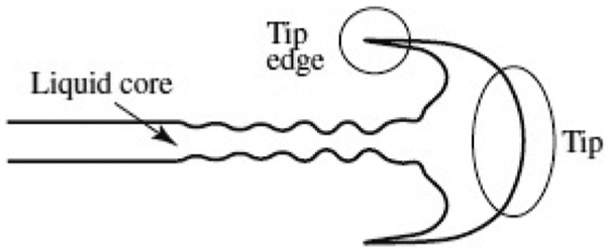
Sketch of the spray case.³

The results produced by the three methods are shown in Figure 2. It can be seen that different methods have their distinct features. The liquid penetration lengths appear to be very similar for the three methods. On comparison of the CLSVOF method (Figure 2(a)) with the Lagrangian method with a break-up model (Figure 2(b)), it is found that, by using the CLSVOF method, more detailed and precise spray break-up dynamics, such as the umbrella-like liquid head formed owing to the liquid jet impact on the ambient gas, can be obtained. At the same time, a few satellite droplets are produced. In contrast, the Lagrangian method generates many small droplets as expected but cannot produce the umbrella-like liquid head. The developed coupled method has the advantages of both the Eulerian method and the Lagrangian method, i.e. high accuracy and low cost, as shown in Figure 2(c). The full circles represent the Lagrangian droplets. The small difference between the droplet distributions in Figure 2(a) and Figure 2(c) is due to the difference between the Lagrangian drag force modelled by equation (8) and the surface tension force modelled by equation (3) in the Eulerian method. Therefore, the current Lagrangian drag force model can be used to model the droplet motion after the Eulerian–Lagrangian transition. More detailed analysis will be presented in the following section. It can be seen from Figure 2 that, although only the spray results in the near-nozzle dense spray region are compared, both the advantages and the disadvantages of the Eulerian method are clearly demonstrated. The motivation of the present study is to develop a hybrid method that combines the Eulerian method and the Lagrangian method and can utilise fully the advantages of both methods, while discarding their disadvantages, as shown in Figure 2(c).

Figure 2.

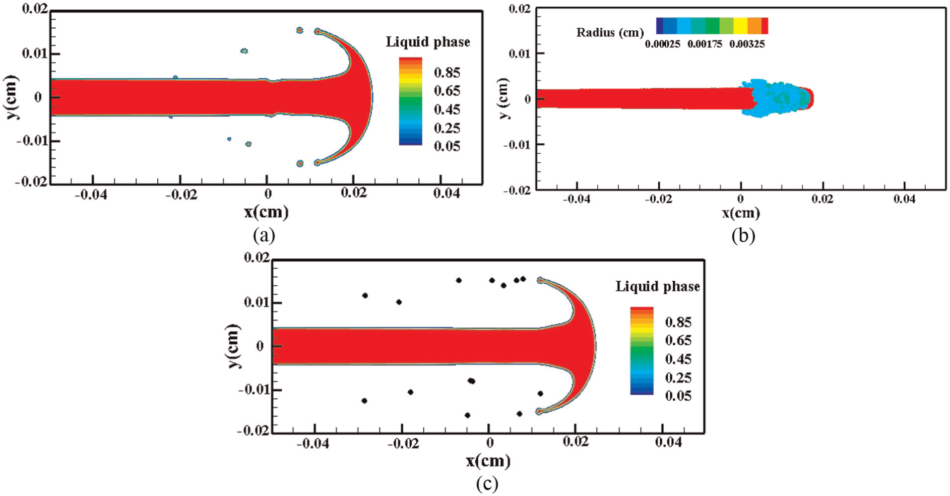
Comparison between the CLSVOF method, the KIVA method and the developed coupled method at 23.6 μs: (a) the Eulerian method; (b) the Lagrangian method; (c) the coupled method. The colour labels represent the liquid-phase volume fractions in (a) and (c), and the droplet radii in (b).

Eulerian–Lagrangian transition

As mentioned in the second section, in order to achieve the Eulerian–Lagrangian transition, three steps are necessary. Figure 3 presents the transition process in detail. According to the neighbour-searching algorithm, different liquid areas are identified by tagging them with different numbers, as shown in Figure 3(a). In Figure 3(b), the isolated small droplets meeting the transition criterion are removed from the Eulerian description.

Figure 3.

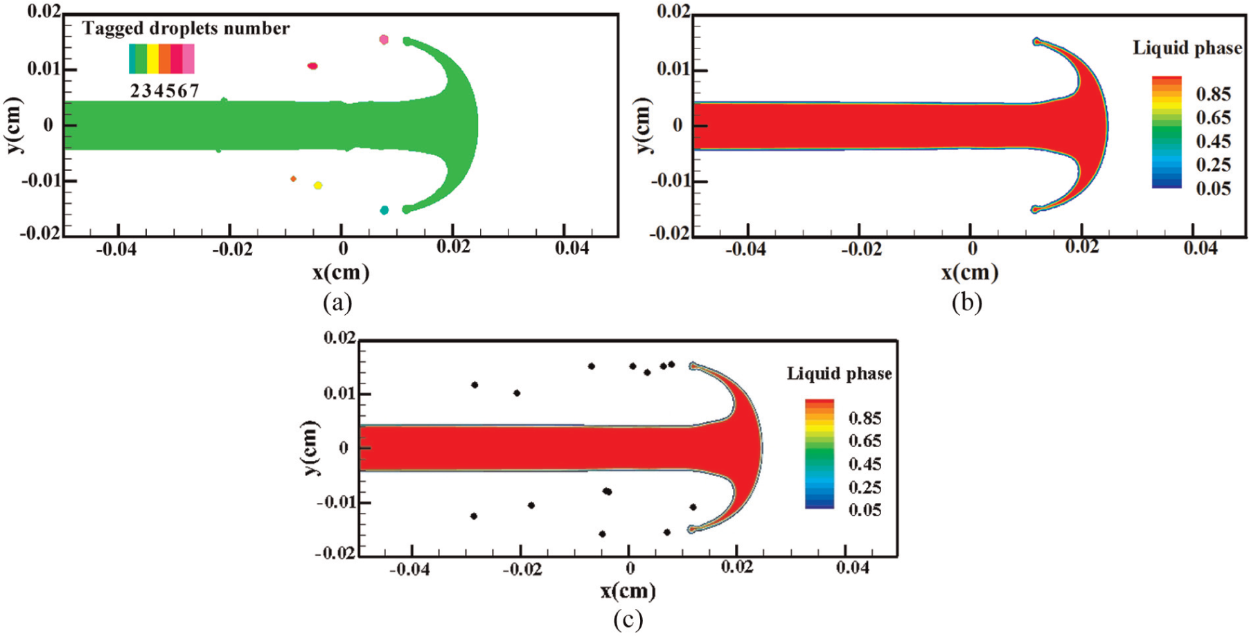
Three steps of droplet transition from using the Eulerian method to the Lagrangian method at 23.6 μs: (a) tagging isolated droplets; (b) removing small isolated droplets; (c) generating Lagrangian particles (full circles) on the KIVA coarse grid.

To check the quality of the numerical transition process, Figure 4 shows a comparison of the droplet masses and the droplet momenta before and after the transition procedure. Figure 4(a) presents the evolution of the change in the overall liquid mass with time. It can be seen that the coupled method and the Eulerian method have the same overall liquid masses. Figure 4(b) and (c) demonstrate the accuracy of the transition process by checking the conservation of the mass and momentum of isolated droplets before and after the transition. The results in Figure 4 demonstrate that in the transition process there is no loss in the droplet mass and no loss in the droplet momentum.

Figure 4.

Mass and momentum conservation before and after the Eulerian–Lagrangian transition: (a) overall liquid mass; (b) masses of isolated droplets; (c) momenta of isolated droplets.

Figure 5 shows the temporal evolution of the liquid jet after t = 18.8 μs. The isolated droplets in Figure 5(a) and (b) are Eulerian droplets and Lagrangian particles respectively. It can be seen that the overall evolution behaviours of the liquid jet are similar, including the distribution of droplets. In the Eulerian method, the interface-tracking algorithm can accurately represent liquid–gas interfaces, their positions and their geometries. However, when the droplet size become very small, resolving these small droplets requires very fine grid resolutions, which greatly increase the computational cost. Therefore, small droplets and thin ligaments are hard to track in the Eulerian framework with any fixed grid resolution. Irrespective of how small the grid resolution is, droplets and ligaments with sizes smaller than the resolution cannot be supported by the grid. On the other hand, the Lagrangian method can deal with these small droplets in a very straightforward way by transferring those small droplets that cannot be supported by the local grids to Lagrangian droplets. Since small droplets solved by the Eulerian method can be transformed into Lagrangian point particles, the requirement of grid resolution can be lowered. This is a critical advantage of the coupled method. Thus, in Figure 5(b) the isolated droplets of different sizes are tracked using the Lagrangian method. For the Eulerian droplets in Figure 5(a), the small droplets that cannot be supported by the grid were removed, as a common procedure in a Eulerian method. It also can be seen that at 21.7 μs the two small droplets come into contact with the liquid core. Since the two droplets are very small and cannot be supported by the CLSVOF method, i.e. they do not satisfy the second condition, we do not consider the reverse Lagrangian–Eulerian transition.

Figure 5.

Comparison between the two-dimensional spray results obtained by the Eulerian method and obtained by the coupled method: (a) Eulerian droplets obtained by the CLSVOF method; (b) Lagrangian particles obtained by the coupling method.

In order to check further the quality of the transition process in a quantitative way, the instantaneous positions of the Eulerian droplets and the Lagrangian droplets are compared in Figure 7. In order to perform this comparison, the trajectories of Eulerian droplets are also tracked. Figure 6 shows the tracking algorithm for the Eulerian droplets. The two important parameters are the volume of droplets and the position of the centre of the droplet mass. The tracking list is empty initially, and isolated droplets can be directly added to the tracking list. At every time step, comparison of the volume and the position of the droplets at the current time step with those in the tracking list at the last time step is performed. If the difference is small, it can be deduced that they are the same droplet. Then, the information on the droplet in the tracking list is updated using the information at the current time step. If there is no matched droplet in the tracking list, the droplet is recognised as a new droplet and directly added to the tracking list. Once the droplet is added to the tracking list, it has a unique constant number to identify it. It is worth noting that tracing isolated Eulerian droplets costs computational time because of the large deformation of droplets induced by the surface tension force.

Figure 6.

The Eulerian-droplet-tracking algorithm.

Figure 7.

Comparison between the droplet positions with time obtained by the Eulerian CLSVOF method and those obtained by the coupled method.

Using the above tracking algorithm, Figure 7 shows the comparison between the instantaneous positions of isolated droplets obtained by the Eulerian CLSVOF method and those obtained by the coupled method. The four isolated droplets can be clearly seen in Figure 5(b) (Lagrangian particles). The trajectories of the four droplets tracked by the coupled method agree well with those tracked by the Eulerian method. Figure 7 also indirectly demonstrates that the drag force model used in the Lagrangian method is appropriate and acceptable under the conditions in this work. The small difference between the coupled method and the Eulerian method is partly because of the deformation and numerical break-up of droplets, and partly because the drag coefficient in the Lagrangian method should be used for a spherical droplet, but the current simulations are two dimensional. However, within the Reynolds number range of 30–80 for the current droplets, the difference is very small. Note that the Lagrangian droplets are solved on a coarser grid, and the Eulerian droplets are tracked on a finer grid, which indicates that the coupled method is able to reduce the computation cost in this work.

Lagrangian–Eulerian transition

The section on the Eulerian–Lagrangian transition considered the transition from a Eulerian droplet to a Lagrangian point particle. The reverse process is also important in many cases. In a complex spray process modelled by a hybrid Eulerian–Lagrangian method, all the interactions (i.e. between the Eulerian droplets and the Eulerian droplets, between the Eulerian droplets and the Lagrangian droplets and between the Lagrangian droplets and the Lagrangian droplets) need to be carefully considered. The section on the Lagrangian–Eulerian droplet transition in this paper presents a method of transforming a Lagrangian particle to a Eulerian droplet to cope with interactions between the Eulerian droplets and the Lagrangian droplets.

Figure 8 illustrates the transition from a Lagrangian particle shown as a full circle to a Eulerian droplet. Before the transition the Lagrangian particle is in contact with the liquid core, which means that the distance of the centre of mass of the droplet to the liquid jet core surface is equal to or smaller than the droplet radius, and the Lagrangian droplet volume is larger than V _2 × 2E. The transition criteria are met. Thus, first, the Lagrangian droplet is removed from the Lagrangian droplet list, as shown in Figure 8(b). Then, a Eulerian droplet is formed (Figure 8(c)). Thus, the entire transition process is completed. It is worth noting that the current Lagrangian–Eulerian transition considers the scenario when only one Lagrangian droplet hits the liquid core, but the transition algorithm can be applied and extended to other complex situations. Figure 9 checks the mass conservation quality of the transition process. It can be seen that the droplet masses are very similar before and after the transition process.

Figure 8.

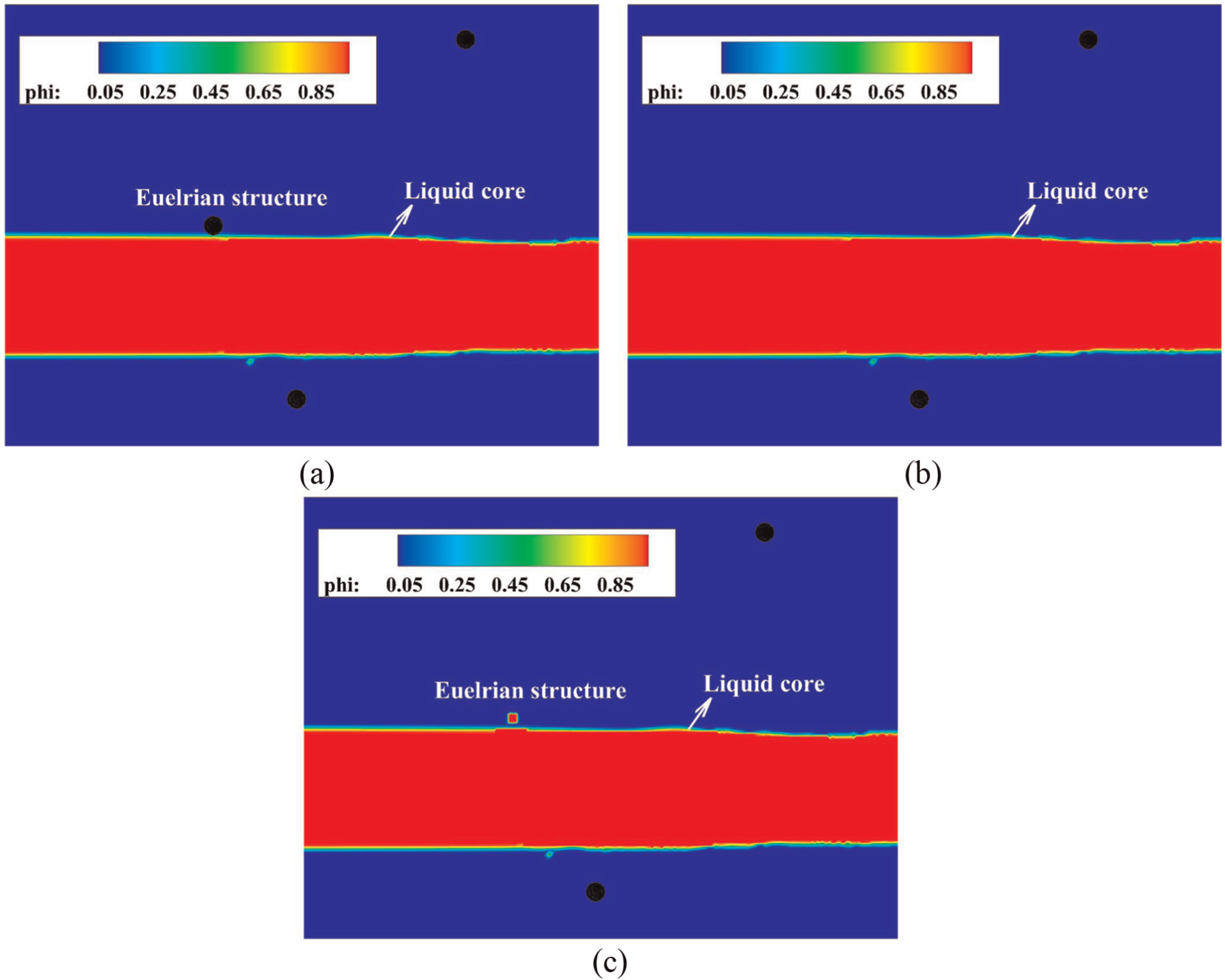
The Lagrangian–Eulerian transition process: (a) before transition; (b) removal of the Lagrangian droplet; (c) transition to the Eulerian droplet.

Figure 9.

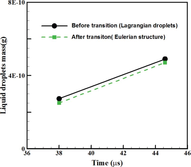
Mass conservation before and after the Lagrangian–Eulerian transition.

Conclusion

This paper presents a multi-scale hybrid Eulerian–Lagrangian approach to simulating liquid jet atomisation processes. The coupled algorithm and procedure are presented in detail. The detailed transition process from using the Eulerian method to using the Lagrangian method to track a small droplet is conducted in three steps. The instantaneous droplet mass and momentum are found to be conserved before and after the transition. We developed a tracking algorithm for droplets tracked in the Eulerian framework for comparison with the droplet motion modelled in the Lagrangian framework. We successfully obtained good agreement on the droplet trajectories, which confirms that the Eulerian–Lagrangian transition method is sound and suitable for the coupling between the Eulerian CLSVOF method and the Lagrangian point-particle method. In addition, the transition process from a Lagrangian particle back to a Eulerian droplet is also considered. In our future work, secondary break-up, collision and coalescence, and evaporation of Lagrangian particles will be considered to improve further the capacity of the multi-scale method to simulate spray processes.

Footnotes

Declaration of Conflicting Interests

The author(s) declared no potential conflicts of interest with respect to the research, authorship, and/or publication of this article.

Funding

The author(s) disclosed receipt of the following financial support for the research, authorship, and/or publication of this article: This work was supported by the Engineering and Physical Sciences Research Council of the UK (grant number EP/L000199/1).

References

Lebas

Menard

Beau

. Numerical simulation of primary break-up and atomization: DNS and modelling study. Int J Multiphase Flow 2009; 35: 247–260.

Hoyas

Gil

Margot

. Evaluation of the Eulerian–Lagrangian spray atomization (ELSA) model in spray simulations: 2D cases. Mathl Comput Modelling 2013; 57: 1686–1693.

Shinjo

Umemura

. Simulation of liquid jet primary breakup: dynamics of ligament and droplet formation. Int J Multiphase Flow 2010; 36: 513–532.

Jiang

Siamas

Jagus

Karayiannis

. Physical modelling and advanced simulations of gas–liquid two-phase jet flows in atomization and sprays. Prog Energy Combust Sci 2010; 36: 131–167.

Lee

Park

. Characterization of the spray atomization process of a multi-hole gasoline direct injector based on measurements using a phase Doppler particle analyser. Proc IMechE Part D: J Automobile Engineering 2013; 227(7): 951–965.

Dimitriou

Peng

Wang

. Effects of advanced injection strategies on the in-cylinder air–fuel homogeneity of diesel engines. Proc IMechE Part D: J Automobile Engineering 2015; 229(3): 330–341.

Hoyas

Pastor

Khuong-Anh

. Application and evaluation of the Eulerian–Lagrangian spray atomization (ELSA) model on CFD diesel spray simulations. SAE paper 2011-37-0029, 2011.

Xia

Luo

Zhao

. Dynamic large-eddy simulation of droplet effects on a reacting plume in countercurrent configuration. Combust Sci Technol 2011; 183: 487–518.

Desjardins

Moureau

Pitsch

. An accurate conservative level set/ghost fluid method for simulating turbulent atomization. J Comput Phys 2008; 227: 8395–8416.

10.

Gorokhovski

Herrmann

. Modeling primary atomization. A Rev Fluid Mech 2008; 40: 343–366.

11.

Wang

Lee

Reitz

Diwakar

. Numerical simulation of diesel sprays using an Eulerian–Lagrangian spray and atomization (ELSA) model coupled with nozzle flow. SAE paper 2011-01-0386; 2011.

12.

Arienti

Soteriou

. Coupled level-set/volume-of-fluid method for simulation of injector atomization. J Propulsion Power 2012; 29: 147–157.

13.

Soteriou

. High-fidelity simulation of fuel atomization in a realistic swirling flow injector. Atomization Sprays 2013; 23: 1049–1078.

14.

Herrmann

. A parallel Eulerian interface tracking/Lagrangian point particle multi-scale coupling procedure. J Comput Phys 2010; 229: 745–759.

15.

Tomar

Fuster

Zaleski

Popinet

. Multiscale simulations of primary atomization. Comput Fluids 2010; 39: 1864–1874.

16.

Vallet

Burluka

Borghi

. Development of a Eulerian model for the “atomization” of a liquid jet. Atomization Sprays 2001; 11: 619–642.

17.

Osher

Fedkiw

. Level set methods: an overview and some recent results. J Comput Phys 2001; 169: 463–502.

18.

Sussman

Puckett

. A coupled level set and volume-of-fluid method for computing 3D and axisymmetric incompressible two-phase flows. J Comput Phys 2000; 162: 301–337.

19.

Capecelatro

Desjardins

. An Euler–Lagrange strategy for simulating particle-laden flows. J Comput Phys 2013; 238: 1–31.

20.

Losasso

Fedkiw

Osher

. Spatially adaptive techniques for level set methods and incompressible flow. Comput Fluids 2006; 35: 995–1010.

21.

Herrmann

. A balanced force refined level set grid method for two-phase flows on unstructured flow solver grids. J Comput Phys 2008; 227: 2674–2706.

22.

Brackbill

Kothe

Zemach

. A continuum method for modeling surface tension. J Comput Phys 1992; 100: 335–354.

23.

Amsden

. KIVA-3V: a block-structured KIVA program for engines with vertical or canted values. Report LA-13313MS, Los Alamos Laboratory, New Mexico, USA, 1997.

24.

Zhou

Luo

Shuai

Xie

. Large-eddy simulations of diesel spray with a fine grid in a constant-volume vessel. Proc IMechE Part D: J Automobile Engineering 2015; 229(2): 247–260.

25.

Nordin

. Complex chemistry modeling of diesel spray combustion. PhD thesis, Chalmers University of Technology, Sweden, 2001.

26.

Liu

Mather

Reitz

. Modeling the effects of drop drag and breakup on fuel sprays. SAE paper 930072, 1993.