Sage Journals: Discover world-class research

Abstract

This article presents a new method to evaluate the geometry of dull cutting tools in order to verify the necessity of tool re-sharpening and to decrease the tool grinding machine setup time, based on a laser scanning approach. The developed method consists of the definition of a system architecture and the programming of all the algorithms needed to analyze the data and provide, as output, the cutting angles of the worn tool. These angles are usually difficult to be measured and are needed to set up the grinding machine. The main challenges that have been dealt with in this application are related to the treatment of data acquired by the system’s cameras, which must be specific for the milling tools, usually characterized by the presence of undercuts and sharp edges. Starting from the architecture of the system, an industrial product has been designed, with the support of a grinding machine manufacturer. The basic idea has been to develop a low-cost system that could be integrated on a tool sharpening machine and interfaced with its numeric control. The article reports the developed algorithms and an example of application.

Keywords

Tool wear tool geometry artificial vision

Introduction

Machining is one of the most used operations in the mechanical workshops because of the high quality of the surface that could be obtained at a competitive price.¹ A driver for the quality of the operation is the integrity of the tool used, both in terms of wear and tooth breakage. The wear of the tooling is influenced greatly by the cutting speed, engagement condition, and speed-dependent cutting force coefficient that are responsible for different cutting forces^2–4 and so tool wear. When an excessive tool wear is detected, the tool is changed and the cutting inserts are substituted or the edges are re-sharpened. The last is a required operation especially for large diameter and high-cost special tooling,⁵ such as the ones commonly used in the die and mold business sector, where the exact geometry of the tool is a critical factor.⁶ In tool sharpening operations performed in mechanical production shops, the machine setup step takes the most of the operation time. The reason is the quite different geometry of the tooling that must be processed by the grinding machine. The tool re-sharpening operation, to be really effective and maintain a long tool life, needs as the input the exact values of the geometrical parameters of the tools. Large companies, which have a great number of tools to be sharpened and small tool variability, usually store the original geometrical data in a database to be accessed before the sharpening operation. In this case, the tool room management system must store the initial geometrical values and the tool must be accurately tracked to update its actual values after every regrinding. If performed manually, such procedure would require high-skill personnel and sophisticated instruments. This makes the work of a regrinding company very complex and time-consuming. The main reason for the complexity of the process is that an accurate measurement procedure is necessary and this is achieved almost always manually by the operators. The regrinding cost for a special tool, in which the geometry is not stored in an electronic format, is very high; this is the case of a lot of small and medium mechanical components’ manufacturers that have a very large tool geometry variability and nearly unique tools. Our aim is to create a simple, automated, and low-cost measurement system capable of providing the following functions:

Measurement of helix and rake angles.

Evaluation of the material to be removed in grinding.

This approach finds its natural application in the re-sharpening high-speed steel (HSS) or solid carbide tools for end milling. Several tool condition monitoring systems (TCMS)^7,8 allow the detection of when the tool must be re-sharpened, but only few⁹ present how to determine the tool geometry and the tool wear or breakage entity. The method chosen to achieve these goals is the artificial vision based on laser line scanning.

This is mainly constituted by a laser line projector, a pair of high-resolution cameras, and a rotating tool holder. The images of the deformed laser line projected on the tool are periodically sampled and stored; a dedicated software extracts from these images a point cloud referred to a unique reference system. Starting from this point cloud, the developed algorithm is able to reconstruct the tool geometry and, by the comparison with previous measurements, to determine the wear profile. This allows the automated setup of the regrinding machine with a considerable operative time reduction for the whole process.

Laser line scanning system is a well-known technique that is commonly used in reverse engineering of medium- to high-size products with form surfaces. In this case, it is possible to adapt this approach to the surface reconstruction of end mills with some minor changes that will be explained in the following paragraphs. The advantages of this technology are mainly the fast acquisition rate and the simplicity and low cost of the system.

The reconstruction accuracy of laser line scanners depends on a set of cross-related issues such as calibration,¹⁰ camera resolution, optics distortion, and noise, while the range acquisition time is dependent on the image processing algorithm. A review on laser scanning methods can be found in the article of Forest and Salvi.¹¹ For measuring an object using a laser line scanner, the following constraints need to be satisfied:

Field of view (FOV): the measured object should be located within the pyramid of the visible zone of the camera defined by the visualization angles of the optic; moreover, the object should be as large as possible in order to utilize completely the camera resolution.

Depth of view (DOV): the measured points should be within a specified range of distance from the cameras in order to produce focused images.

The tool has to be positioned on the rotary table in order to let all the tool surfaces to be scanned by the laser line; no “unexplored regions” have to be allowed on the tool surface.

There exist several other factors such as roughness and reflectance of a surface and ambient illumination that influence the accuracy of the scanning results. Figure 1 graphically illustrates the above-mentioned constraints for the scanning that are needed for measuring a point on a surface.

Figure 1.

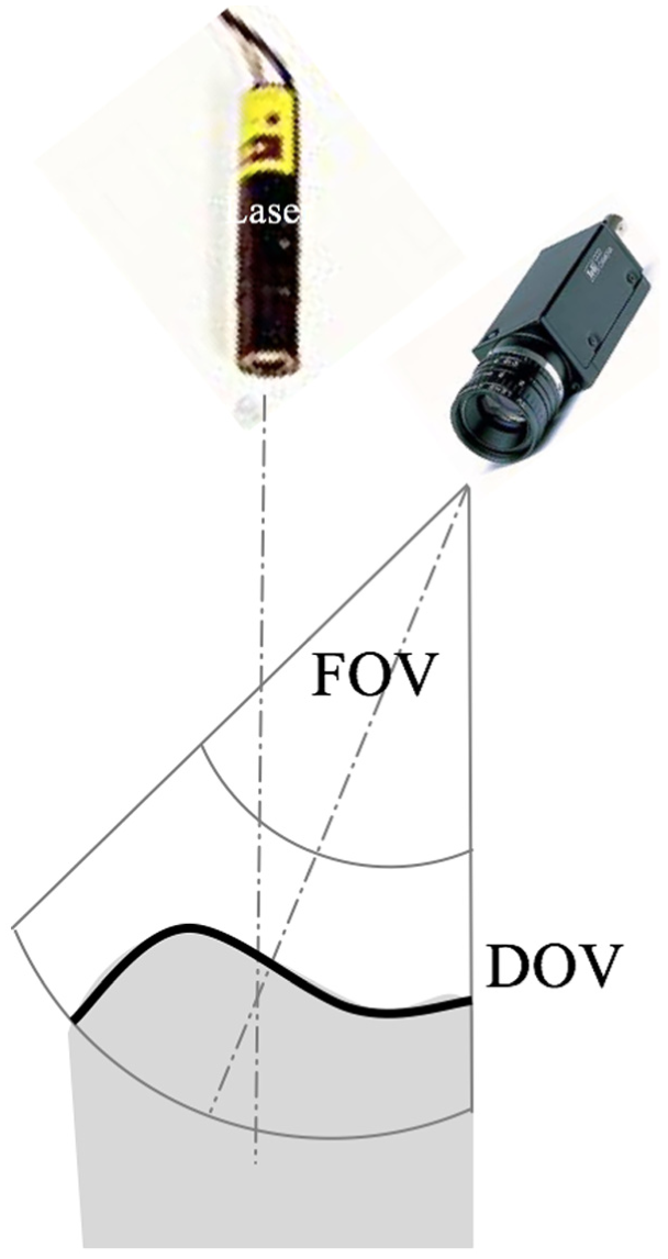
Scanning constraints for a surface using a traditional CCD camera.

The optical properties of the surface significantly determine the performance of the laser scanner, so only certain surfaces can be studied with these techniques. The optimal surface type for scanning purposes is a totally Lambertian surface with a high reflection index. Figure 2(a)–(c) shows, respectively, how a light ray behaves under a specular, Lambertian, and translucid surface. Figure 2 shows also a real case of a laser line on a translucid and Lambertian surface as seen by the camera of the system. The translucid surface produces a lot of undesired light peaks where they are not expected to be and the light power is lowered so the reconstruction quality degrades.

Figure 2.

Different behavior of the laser line on (a) specular, (b) Lambertian, and (c) translucid surface.

In the specific field of cutting tools, translucid surfaces are never found, but often it happens in the case of specular (reflective) surfaces while a Lambertian surface, the best case, is not so common. In order to obtain better results, it is a good practice to clean and dry the tool; this usually limits the probability to have a reflected laser light; however, if these actions are not enough to achieve a satisfying image quality, it is possible to coat the tool with a sprayed matt white paint.

System architecture

The system architecture has been chosen considering the peculiar characteristic of cutting tools such as drills or end mills. The constraints of the design process are the following:

The cameras have to be placed and their optics chosen in order to let all the tools inside their DOV and FOV simultaneously; the setup of the system depends on the general dimension of the tools to be measured.

The optical axis of the cameras is directed in such a way that a point on the tool rotation axis at the table level has its image at the edge of the CCD sensor. This solution maximizes the utilization of the CCD, thereby decreasing the ratio real space metric/CCD pixel that is responsible for the resolution of the system.

Using only one camera would be insufficient for the measurement because in certain cases, it may happen that the points of the tool occlude the vision of the laser line (Figure 3); the problem is solved with two cameras symmetric with respect to the laser plane.

The system must have a production cost of each unit compatible with the cost of the associated regrinding machine and the related selling volume; other more expensive solutions could not find a satisfying market interest; the components have to be chosen accordingly with these constraints.

Figure 3.

Architecture of the system.

The proposed system architecture is reported in Figure 3. The use of two cameras assures the completeness of information and improves the measure precision when the projected laser line is seen by both the cameras. In this case, the information of the two cameras, where redundant, are averaged in order to obtain a higher measure confidence.

Analysis software developed

The software has been developed by the authors in MATLAB^® environment. The starting point has been the definition of a set of requirements, acquired thanks to the collaboration of an Italian tool grinding machine manufacturer; a quality function deployment (QFD) approach has been used to collect information.¹² These could be summarized in the following list:

Automatic determination of some default tool angles; these are helix angle and front and back rake angles for each tooth

Reliability of determination of other geometrical characteristic, that is, tool diameter at every tooth, tool cross section, and so on

Interface with the regrinding machine tool numeric control (NC)

Easy to use

Must work on a common industrial PC processing the images in a time less than 10 s

The processing phases to obtain geometrical information regarding the tool are the following:

The tool is rotated around its axis and every 0.2° to 2° (depending on the precision needed and the tool diameter) two images are acquired by the cameras; each image contains a line; that is the image of the laser line projected on the tool surface. This line is characterized by a thickness variable along the line due to the geometry of the tool. These images are then pre-processed with an algorithm to optimize the contrast and eliminate the pixel not related to the projected laser line using an automatic threshold.

The images are then registered (coupled together after a rotation and a shifting; this is easily done thanks to the angles between the camera and the laser source which are symmetric, +45° and −45°); the result is a unique image that contains the information from both cameras.

The information is then extracted by the image using the most functional algorithm depending on environment light condition. The result is a line of points that represent the coordinates of the laser line projected on the tool.

The process is repeated for each angular position of the tool until the whole surface has been acquired by the system.

The geometric information of the tool is then extracted from the point cloud. The choice has been to use algorithms that use sections of the point cloud instead of strategies based on the study of the full point cloud to extract and study edges. This is due to the minor computational resource needed for the first analysis and the greater ability to study worn profile (edge reconstruction after wear is easier on a profile instead than on a full point cloud). The sections are taken with planes orthogonal to the tool axis.

One section is enough to calculate the rake angles.

Two sections allow to calculate the helix angle.

More sections allow to verify the constancy of the geometrical parameters, to observe tool wear,¹³ or to verify the correct re-sharpening of the teeth.

Line analysis algorithm

The image of the laser light projected on the tool surface is a line characterized by a non-constant width in terms of pixels and with variable brightness. The objective of the first step of analysis is to obtain only a single line of pixels that represent the projection of the laser line on the cutting tool. To perform this reduction, two solutions are available: the first is constituted by a width reduction of the laser line acquired with the image through a thinning algorithm,¹⁴ and the second one is based on the reconstruction of the Gaussian light intensity profile in the line. Since the energy pattern of a laser beam corresponds to a Gaussian profile for most common lasers and the cylindrical lens does not affect such distribution in the lateral direction, the line brightness distribution in the direction perpendicular to the line could be assumed equal to the original power distribution. The maximum intensity points of many transverse sections of the line define the profile of the object to be acquired.

The advantage of the first solution is a lower computational time that, however, produces a lower reconstruction precision. The second approach grants a higher precision at the cost of more computational time; moreover, this solution could be applied only when the laser light intensity is low in order not to saturate the pixel intensity along the width of the line. The lower power of the laser source, however, allows the use of this solution only in case of strongly controlled environmental light condition (nearly dark), which usually could be attained only in a laboratory and not on a system mounted on a production machine in the shop. An example of light intensity saturation in normal environmental light condition is presented in Figure 4.

Figure 4.

Light saturation case in normal environmental condition.

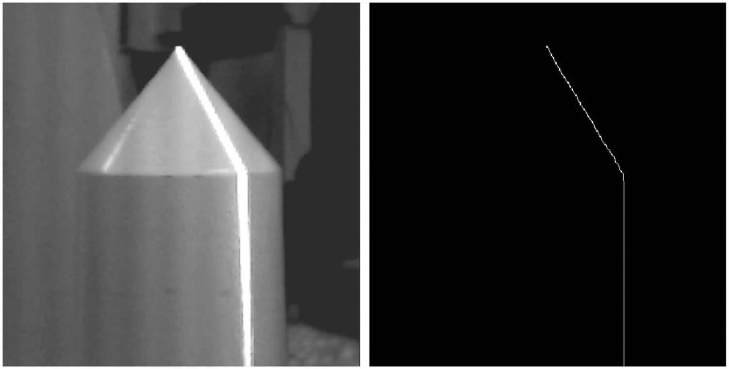
The thinning process is constituted by three phases: an automatic threshold is applied to the image in order to cancel all the characteristics of the background; the images coming from the two cameras are then merged together in order to increase the accuracy and also reconstruct the partially hidden parts and the thinning algorithm is applied to reduce the laser line image to a single line of pixels. The thinning algorithm chosen is based on the original proposal developed by Zhang and Suen:¹⁵ this uses a 3 × 3 convolution matrix that, with an iterative approach, modifies the image till the line is reduced to a single pixel width (Figure 5).

Figure 5.

Example of thinning for a line acquired on a two-tooth milling tool.

The Gaussian approach is based on the computation of the approximating normal distribution of the light intensity profile and the evaluation of the maximum of this curve. At this stage, the state-of-the-art algorithms for the peak position computation are based on the analysis of each row of the image. This approach gives erroneous results when the laser line is nearly horizontal (this error it is consistent till angle of 30°). A new peak computation algorithm has been developed to overcome this problem: the algorithm analyses the laser line and calculates the normal direction for each point. This direction is then used to resample a row of pixel from which the Gaussian peak is computed. This approach provides a series of pixel characterized not by integer coordinates allowing a sub-pixel resolution. It is generally verified that the sub-pixel maximum resolution using Gaussian reconstruction approach could be 1/32nd of pixel.

Both the algorithms have been implemented and tested, and for the machine to be constructed the first solution has been chosen in order to provide a more robust system with only a small decrease in the maximum precision obtainable. The second solution could be applied in case of greater precision needed when the computational time is not a constraint of the problem and the machine could be modified in order to isolate the measuring zone from environmental light.

Triangulation algorithm

The single line of pixels produced by the thinning algorithm is processed by a triangulation routine, with the aim to relate every pixel of each two-dimensional (2D) image to a point in a three-dimensional (3D) coordinate space. Every pixel, thanks to three triangulation equations, is converted into a 3D coordinate point. In order to fully define these coordinates, it is also necessary to relate each pixel line to a specific angular position of the tool (to reconstruct the whole tool surface, the tool is rotated around its axis). The acquisition and processing of the couples of images are performed for each defined angular step. With this strategy, it is possible to reconstruct a “point cloud” that represents the tool geometry. The triangulation equations, used by the authors for this use case, are the following

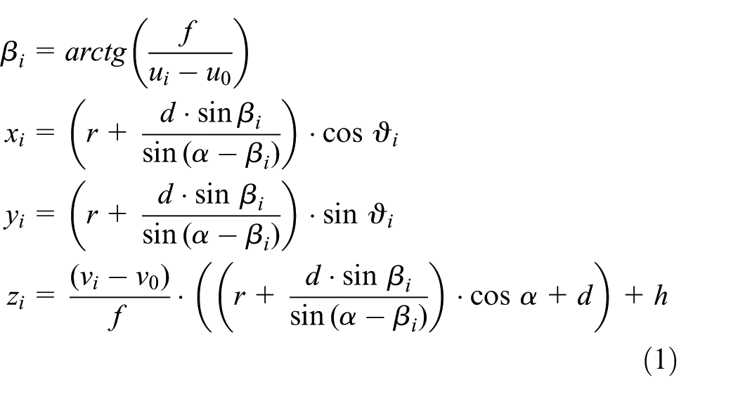
\begin{matrix} β_{i} = a r c t g (\frac{f}{u_{i} - u_{0}}) \\ x_{i} = (r + \frac{d \cdot \sin β_{i}}{\sin (α - β_{i})}) \cdot \cos ϑ_{i} \\ y_{i} = (r + \frac{d \cdot \sin β_{i}}{\sin (α - β_{i})}) \cdot \sin ϑ_{i} \\ z_{i} = \frac{(v_{i} - v_{0})}{f} \cdot ((r + \frac{d \cdot \sin β_{i}}{\sin (α - β_{i})}) \cdot \cos α + d) + h \end{matrix}

(1)

where α is the angle between the axes of the camera and the laser source; f is the focal length of the camera; d is the distance between the optical center of the camera and laser plane; ϑ_i is the progressive rotation angle of the tool; u_i and v_i are the horizontal and vertical coordinates of a pixel of the acquired line on the image, respectively; u₀ and v₀ are the coordinates of the center of the pixel sensor; x_i, y_i, and z_i are the coordinates of the pixel in the real space coordinate system; and r and h are the x- and z-coordinates of a point seen in the central pixel of the charge-coupled device (CCD) sensor, respectively, on the laser plane and on the rotary table axis. The 3D space coordinates (x, y, z) are the three orthogonal axes, right-handed, where z coincides with the rotation axis and x is the laser direction with ϑ = 0 while the origin is on the rotary table top. The origin of the u, v coordinates on the image sensor is defined by the image of a point on the rotation axis placed at the rotary table level.

A schematic representation of the system is presented in Figure 6.

Figure 6.

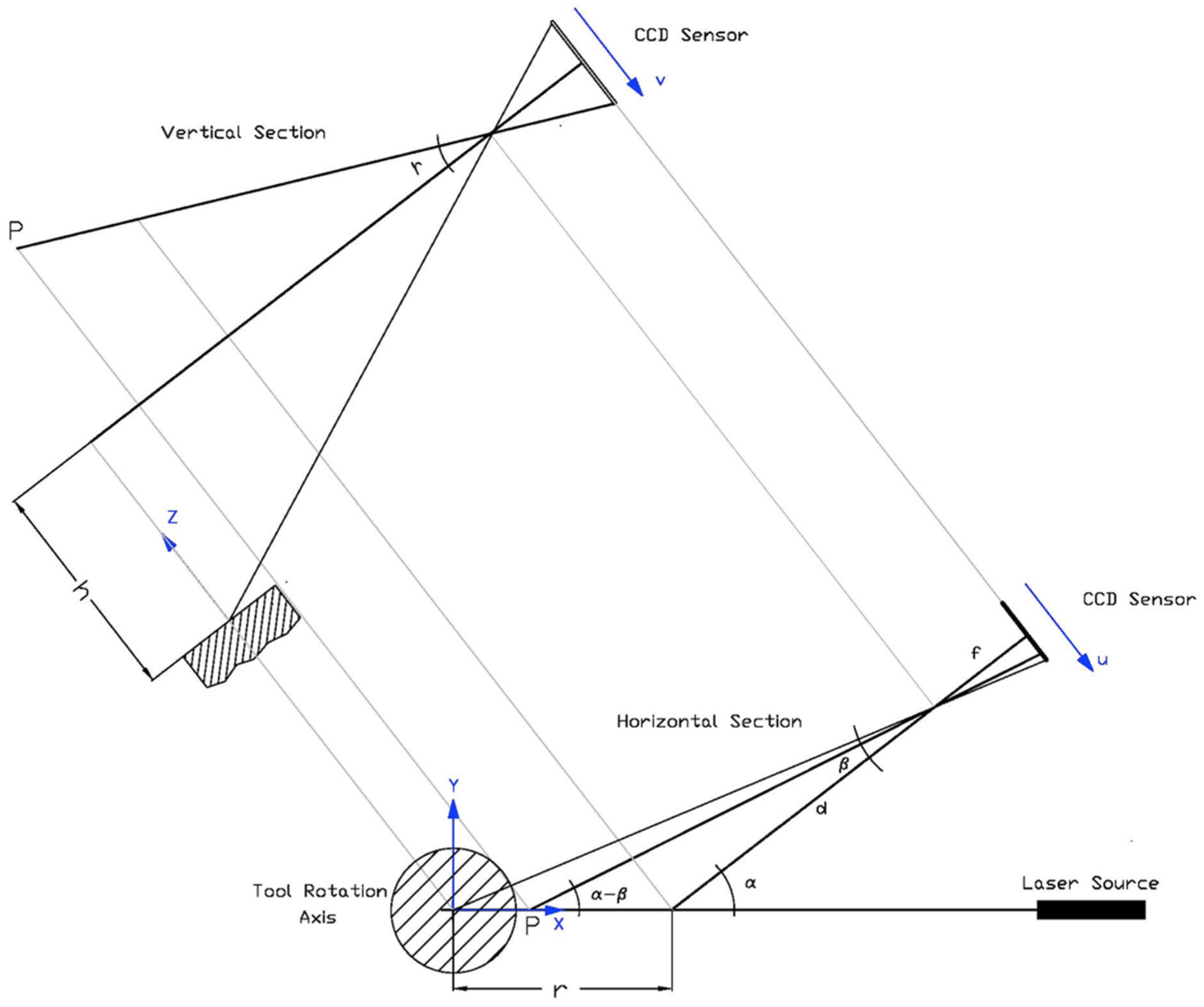
Schematic representation of the system.

Sectioning the point cloud and edge reconstruction

The tool surface contains creases and corners, so it is necessary to find the feature lines and junctions beforehand.^16,17 Many algorithms and approaches have been developed to satisfy this need. The graph-based surface reconstruction of Bleyer and Gelautz¹⁸ handles sharp edges by maximizing for each point the sum of dihedral angles of the incident faces. The optimization is performed only locally and depends on the order in which the input points are processed. Adamy et al.¹⁹ described corner and crease reconstruction as a post processing step of finding a triangulation describing a valid approximating surface. The power crust algorithm of Amenta et al.²⁰ treats sharp edges and corners also in a post processing step. Guy and Medioni²¹ describe a robust algorithm to extract surfaces, feature lines, and feature junctions from noisy point clouds. They discretize the space around the point cloud into a volume grid (voxel representation) and accumulate for each cell surface vote from the data points.

A simplified approach, which has been used in this work, is given by the use of sliced points cloud. When applicable, this approach reduces considerably the complexity of the problem to be solved in order to automatically identify the surface edges. The approach starts from the study of many slices of the point cloud on which it is possible and easy to evaluate features and discontinuities. The features so isolated should belong to more adjacent slices. Several neighboring slices should also contain points that form the same, or at least a similar feature. With a well-structured process, all points in each slice are matched to their corresponding points in the previous slice.

From the edge evaluation, it is necessary to extract the original geometrical cutting angles and an indication of geometrical changes induced by the natural tool wear (NTW).²²

In order to obtain the values of tool angles needed for the re-sharpening process, it is necessary to section the point cloud with planes orthogonal to the tool axis or, if needed, orthogonal to the helix curve in a chosen measuring point. The first problem to be solved is the interpolation of the points on the section plane, because only few (or none) of them will belong to the plane. To solve this problem, it is very useful to maintain, in the point cloud organization, the index of the acquired line (ϑ_i) to which each point belongs. The developed strategy is then to evaluate the nearest points on each radial contour immediately lower and upper with respect to the section plane; the point reported on the plane will be defined by the intersection of the segment that links these two points and the plane itself. The planar section is now described by a sequence of discrete points (for example, 360 points with an angular distance between the images of 1°). An example of this sectioning strategy is presented in Figure 7.

Figure 7.

Example of point cloud sectioning.

This section usually could represent easily the general geometry of the tool, but the exact positions of the sharp edges are usually lost for two main reasons: because it is really unlikely that the laser line exactly crosses the edge at that value of Z and because the wear of the tool has blunted the edges.

Either it is required to measure the tool angles (low-resolution cameras) or evaluate tool wear (high-resolution cameras); the profile is composed of curved and straight lines connected in points where the direction suddenly changes (profile edges). The procedure developed for transforming the point sequence in continuous line and compute the tool angles is as follows:

The zones of the point sequence where the direction changes are roughly recognized using an algorithm that calculates the relative angles among a short series of points.

Discarding some points in the neighborhood of these zones, each substring of pixels is approximated with a B-spline.

The B-splines of the profile are then computed and extended until the intersection with the near ones; these intersections are the sharp edges presumably lost with the profile discretization.

Some tool angles are then computed as the angles among the B-spline of the profile (e.g. rake and front tool angle for a profile perpendicular to the helix curve for an end mill) while other angles have to be computed considering more sections (such as the helix angle whose calculation needs the analysis of more sections) (Figure 8).

Figure 8.

Edge evaluation procedure.

The amount of the material to be removed in grinding is computed using the following procedure:

A number of sections, starting from the tool point, are obtained (Figure 9; the number of sections to be used is reduced only in order to improve the visualization quality).

The profile of the tool for each section is computed and the edges are evaluated.

The same edge is retrieved on the different sections and a planar representation of the edge is created positioning the edge on the same line (Figure 10); this step is necessary for helical tool.

This representation is functional to evaluate the material to be removed from the tool suing different strategies. This will change the regrinding machine setup in terms of depth of cut and offset registration. The best option is to maintain constant the cutting tool length and reduce the diameter (line a in Figure 10 represents the sharpened tool contour); this approach is used for some tools in the die manufacturing sectors. The second option is to maintain the diameter equal to the original one (line b in Figure 10), common solution for contouring tools; in this case, the grinding machine will operate on the side of the tool. The last option is to remove as less as possible material from the tool (line c of Figure 10), without the limitation of maintaining the original length and diameter. In this case, both the face and side of the tool are to be grinded.

Figure 9.

Cutting tool sectioning.

Figure 10.

Choice of the re-sharpening strategies for grinding worn profile: (line a) maintain original tool length, (line b) maintain original external diameter, and (line c) minimum material removal.

User interface

In order to facilitate the use of the system by an inexperienced user, a specific software interface has been developed. From the user interface, it is possible to load or acquire the images of the tool and decide where and how to section the point cloud. The section is then automatically studied in order to evaluate the characteristic tool angles; specific options allow the user to refine the analysis (choice of order or the interpolating spline, threshold angle to recognize an edge, etc.). The user interface produces three different graphical outputs: a representation of the points cloud, a graph of the section points with the reconstructed edge, and finally an interpolated graph of the sections. This last graph is the contour described as a B-spline sequence (Figure 11).

Figure 11.

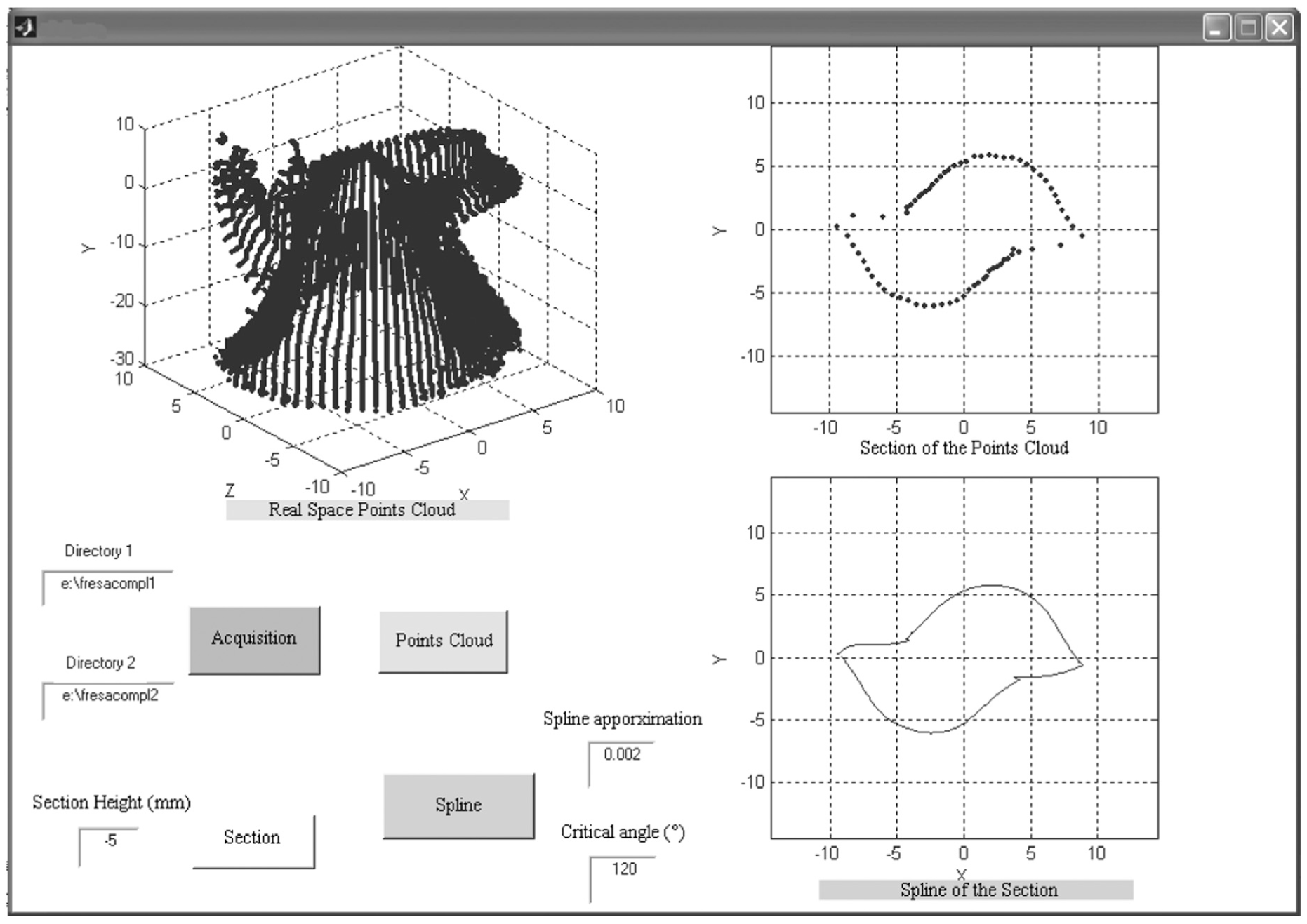
Screenshot of the developed user interface.

System calibration

The accuracy of the system is strongly related to the system calibration. The calibration of the system has the aim to evaluate the optical characteristics of the cameras used (focal length) and their relative position, in relation to the laser line projected and the tool holder. In order to simplify the calibration, the laser line is projected on a target placed on the tool holder in such a way that the projection plane contains the rotation axis. In order to calibrate the system, a simple test for the cameras has been developed. The image of a special tool, a calibrated cylinder, is acquired by the two cameras at different distances. The analysis of the images allows to calculate the focal length (f in (1)) and the distance of the focal point of the camera from the rotation axis (d in (1)). Also, an algorithm to correct the optical distortion of the lenses has been developed based on an optical distortion model^23,24 that corrects radial and asymmetric distortion. To perform such lenses’ correction, it is necessary to acquire many images (about 20) of a calibrated chessboard at various angles. This operation acquires automatically the intersection points of the chessboard and creates a distortion map that will be used by a specific algorithm to correct the image.

Example of application

An example of application for a two-tooth end mill is reported and a comparison of some measures performed with traditional methods is presented in Table 1. Figure 11 presents the point cloud of the two-tooth end mill acquired; the rotational angle step chosen, 5°, is very large in order to produce clear and understandable figures, while in normal working condition lower step angles are suggested (2° is an optimal compromise between time needed for the acquisition and resolution; on a NC machine the process could be easily automated in order to reach even greater detail). The results of the angle computation are reported in Table 1.

Table 1.

Results of the measured tool.

	1° Edge	2° Edge
Diameter of the end mill (mm)	19.29
Distance of tool tip from the rotation axis (mm)	9.65	9.15
Front rake angle (°)	−5.1	−7.6
Back rake angle (°)	45.7	46.1
Tool angle (°)	49.4	51.5
Helix angle (°)	20.1

The same dimensions have been acquired using a DMG Mori UNO setting station, able to acquire the geometrical data of the tooling off-line. The measures have been carried out both on the new and worn tools in order to verify the stability of these measures after the process. The maximum error found between the commercial off-line system and the developed test bench is about 50 µm on the diameter and 1° for the angles.

Working prototype of the product

The tests to obtain the product performance and support the development of the image analysis algorithms have been carried out using a test bench (Figure 12). From the results obtained using the test bench, a final product design has been elaborated, thanks also to the support of BiEmme, a grinding machine manufacturer. The industrial product has been designed to be used on a large variety of regrinding machines, thanks to the simple interface with the machine ram. In order to meet the precision requirements, a set of ad hoc components have been selected. The laser line generator chosen is a min laser with a nominal line width of 10 microns and an homogeneous light intensity across the line length (Lasiris standard). The cameras are two micro vision systems characterized by low cost, good resolution (2560 × 1920), and good optical part (low lens distortion). The final product design is presented in Figure 13.

Figure 12.

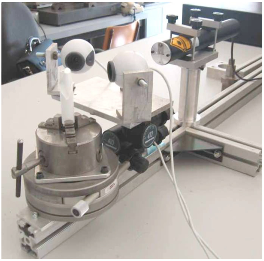
Test bench for the performance estimation.

Figure 13.

Scheme of the product architecture and regrinding machine tool interface.

Conclusion

The vision system equipped with the developed software is able to calculate the re-sharpening angle of a worn tool in order to automate the re-sharpening process. The system developed is able to evaluate the section of the tool at various heights and inclination with a mean uncertainty of about 50 µm. The angle computation has proven an uncertainty of ±1°. Possible improvements have been evaluated during this experience, especially regarding the use of controlled light condition for the image acquisition that could allow the use of more performing image analysis acquisition algorithms tested during the development of the system. An integration of this information with the NC of the machine could allow the development of a “self-setting tool grinder” that could reduce relevantly the time needed for the setup operation.

Footnotes

Acknowledgements

In the development of this research, a special thanks is due to Eng. Massimo Morelli of BiEmme srl, manufacturer of sharpening machine tools, who has provided a relevant support of knowledge and information.

Academic Editor: Xichun Luo

Declaration of conflicting interests

The author(s) declared no potential conflicts of interest with respect to the research, authorship, and/or publication of this article.

Funding

The author(s) received no financial support for the research, authorship, and/or publication of this article.

References

Gupta

Nau

DS.

Interpreting product designs for manufacturability evaluation. New York: Design Engineering Division, American Society of Mechanical Engineers (Publication) DE, 1993, pp.33–43.

Grossi

Sallese

Scippa

. Chatter stability prediction in milling using speed-varying cutting force coefficients. Proced CIRP 2014; 14: 170–175.

Yen

Söhner

Weule

. Estimation of tool wear of carbide tool in orthogonal cutting using FEM simulation. Mach Sci Technol 2002; 6: 467–486.

Grossi

Sallese

Scippa

. Speed-varying cutting force coefficient identification in milling. Precis Eng 2015; 42: 321–324.

Hisataka

Kato

Sugiyama

. Study on re-sharpening technology of ball end mills. In: Proceedings of the 8th international conference on progress of machining technology (ICPMT2006—progress of machining technology), Matsue, Japan, 9–11 November 2006, pp.93–96.

Campatelli

Scippa

A heuristic approach to meet geometric tolerance in high pressure die casting. Simul Model Pract Th 2012; 22: 109–122.

Altintas

Yellowley

In-process detection of tool failure in milling using cutting force models. J Eng Ind: T ASME 1989; 111: 149–157.

Ritou

Garnier

Furet

. Angular approach combined to mechanical model for tool breakage detection by eddy current sensors. Mech Syst Signal Pr 2014; 44: 211–220.

Giusti

Santochi

Tantussi

On-line sensing of flank and crater wear of cutting tools. CIRP Ann: Manuf Techn 1987; 36: 41–44.

10.

Salvi

Armangué

Batlle

A comparative review of camera calibrating methods with accuracy evaluation. Pattern Recogn 2002; 35: 1617–1635.

11.

Forest

Salvi

. A review of laser scanning three-dimensional digitisers. In: IEEE international conference on intelligent robots and systems, Lausanne, 30 September–4 October 2002, pp.73–78. New York: IEEE.

12.

Nahm

Ishikawa

Inoue

New rating methods to prioritize customer requirements in QFD with incomplete customer preferences. Int J Adv Manuf Tech 2013; 65: 1587–1604.

13.

Prasad

Ramamoorthy

Tool wear evaluation by stereo vision and prediction by artificial neural network. J Mater Process Tech 2001; 112: 43–52.

14.

Wang

Zhang

Synthetically thinning algorithm for fingerprint image. Jisuanji Fuzhu Sheji Yu Tuxingxue Xuebao/J Comput-Aided Des Comput Graph 2009; 21: 179–182.

15.

Zhang

Suen

CY.

Fast parallel algorithm for thinning digital patterns. Commun ACM 1984; 27: 236–239.

16.

Algorri

Schmitt

Surface reconstruction from unstructured 3D data. Comput Graph Forum 1996; 15: 47–60.

17.

Boscheri

Dumbser

Righetti

A semi-implicit scheme for 3D free surface flows with high-order velocity reconstruction on unstructured Voronoi meshes. Int J Numer Meth Fl 2013; 72: 607–631.

18.

Bleyer

Gelautz

Graph-based surface reconstruction from stereo pairs using image segmentation. In: Proceedings of SPIE, San Jose, CA, 17 January 2005, pp.288–299. Bellingham, WA: SPIE.

19.

Adamy

Giesen

John

. New techniques for topologically correct surface reconstruction. In: Proceedings of the IEEE visualization conference, Salt Lake City, UT, 13 October 2000, pp.373–380. New York: IEEE.

20.

Amenta

Choi

Kolluri

RK.

The power crust, unions of balls, and the medial axis transform. Comp Geom: Theor Appl 2001; 19: 127–153.

21.

Guy

Medioni

Inference of surfaces, 3D curves, and junctions from sparse, noisy, 3D data. IEEE T Pattern Anal 1997; 19: 1265–1277.

22.

Ding

Zhang

. On-line monitoring for cutting tool wear reliability analysis. In: Proceedings of the world congress on intelligent control and automation (WCICA), Taipei, Taiwan, 21–25 June 2011, pp.364–369. New York: IEEE.

23.

Feng

Liu

Analysis of digitizing errors of a laser scanning system. Precis Eng 2001; 25: 185–191.

24.

Tian

Yang

Zhang

. An experimental evaluation method for the performance of a laser line scanning system with multiple sensors. Opt Laser Eng 2014; 52: 241–249.

Development of an artificial vision system for the automatic evaluation of the cutting angles of worn tools

Abstract

Keywords

Introduction

System architecture

Analysis software developed

Line analysis algorithm

Triangulation algorithm

Sectioning the point cloud and edge reconstruction

User interface

System calibration

Example of application

Working prototype of the product

Conclusion

Footnotes

Acknowledgements

Declaration of conflicting interests

Funding

References