Sage Journals: Discover world-class research

Abstract

A Green’s function method is proposed to calculate transient heat flow through the building wall in this article. In order to obtain a simplified analytical solution for dynamic heat transfer problems, approximation is applied to the solution. And it can also make numerical simulation faster. The approximation solution and the exact solution got by MATLAB are compared under four different heat transfer conditions for a practical problem to verify its accuracy. Furthermore, double layer building wall analysis model is developed for practical application.

Keywords

Green’s function heat transfer transient analysis approximation analytical solution

Introduction

Heat conductivity in a wall is a traditional problem, and there are different numerical methods to solve it, such as finite difference method,^1,2 harmonic method,^3,4 response coefficient method,^5–7 Laplace’s method,^8,9 and Z-transfer function.^10,11 But in some way, they are not easy to use because calculating time is strongly limited by time step and mesh size, regular temperature change is required, accurate coefficients are needed, and analytical solution is not easy to get. So current researchers focus on factors of wall, such as decrement factor and time lag values,¹² static and dynamic thermal characterization,¹³ and response factors (three-dimensional conduction). Green’s function can also be used to solve the problem, but the analytical solution is very hard to use. If proper approximation to the solution is applied, it can also be a powerful tool to solve the problem.

Green’s function was used in many different fields; Haji-Sheikh et al.¹⁴ investigated a Green’s function solution of the thermal wave effect during rapid heating of pure dielectric materials. Mertiny and colleagues¹⁵ developed a Green’s function approach, and it was used to predict the temperature distribution within polymeric substrates during flame spraying. Wang et al.¹⁶ developed a useful method to conduct thermal analysis of insulated steel members exposed to fire. Wang et al.¹⁷ proposed a method to investigate the heat conduction in multilayer solid walls. CAB Vasconcellos et al.¹⁸ elaborated the numerical algorithm based on Green’s function for multilayer systems. This article describes the method in detail (including monolayer and multilayer conditions) and simplifies it based on the way of simplified integral algorithm used in the monolayer condition. This method is also appropriate for the calculation of multilayer walls, as we have tested the method in this research. In the article based on Green’s function, approximation is applied to the solution and makes it available to analysis room’s thermal properties.

Formulation of the problem

The partial heating (i.e. the wall is partly heated or a small part of space is heated) is not considered often for a constant property wall. So it can be regarded as a one-dimensional heat transfer problem. According to Figure 1, it is assumed that the initial temperature distribution of the wall is $F (x)$ and heat fluxes of inside and outside surfaces are $f_{0} (τ)$ and $f_{L} (τ)$ , and the inner heat source can be described as $q_{v} (x, τ) = ρ c_{p} g (x, τ)$ in which $ρ$ and $c_{p}$ are the density and the specific heat capacity of the wall, respectively. Thus, mathematical description of the problem is given as follows

{\begin{matrix} \frac{\partial t}{\partial τ} = a \frac{\partial^{2} t}{\partial x^{2}} + g (x, τ) & 0 < x < L, τ > 0 \\ t = F (x) & 0 < x < L, τ = 0 \\ - λ \frac{\partial t}{\partial x} = f_{0} (τ) & x = 0, τ > 0 \\ λ \frac{\partial t}{\partial x} = f_{L} (τ) & x = L, τ > 0 \end{matrix}

(1)

Figure 1.

Description of the problem.

Green’s function G is established as follows

{\begin{matrix} \frac{\partial G}{\partial τ} = a \frac{\partial^{2} G}{\partial x^{2}} + δ (x - x^{'}) δ (τ - τ^{'}) & 0 < x < L, τ > 0 \\ G = 0 & 0 < x < L, τ = 0 \\ \frac{\partial G}{\partial x} = 0 & x = 0, τ > 0 \\ \frac{\partial G}{\partial x} = 0 & x = L, τ > 0 \end{matrix}

(2)

Assuming that there is no inner heat source in the wall before time $τ'$ and the temperature distribution of the wall before time $τ'$ , the effect of inner heat source is equal to the initial temperature distribution of the wall at the time $τ'$ . Therefore, the problem above could be described as follows

{\begin{matrix} \frac{\partial G}{\partial τ} = a \frac{\partial^{2} G}{\partial x^{2}} 0 < x < L, τ > 0 \\ G = δ (x - x') 0 < x < L, τ = τ' \\ \frac{\partial G}{\partial x} = 0 x = 0, τ > 0 \\ \frac{\partial G}{\partial x} = 0 x = L, τ > 0 \end{matrix}

(3)

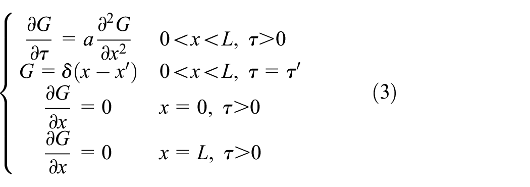
In the above equations, $λ$ and L are the thermal conductivity coefficient and the thickness of the wall, and a is the thermal diffusivity.

Applying the method of separation of variables, coefficients of the solution can be calculated from initial conditions of the equation. Then, Green’s function of the problem can be obtained using Fourier expansion method

\begin{matrix} G (x, τ; x' τ') = \frac{1}{L} + \frac{2}{L} \sum_{m = 1}^{\infty} \exp [- \frac{m^{2} n^{2} a (τ - τ')}{L^{2}}] \\ \cos \frac{m π x'}{L} \cos \frac{m π x}{L} \end{matrix}

(4)

In this problem, the temperature distribution at time $τ$ can be divided into three parts: the temperature distribution, $t_{1} (x, τ)$ , caused by inner heat source, the temperature distribution, $t_{2} (x, τ)$ , caused by initial temperature distribution, and the temperature distribution, $t_{3} (x, τ)$ , caused by heat fluxes of surfaces.

In this problem, there is no inner heat source in the wall, so

t_{1} (x, τ) = 0

The temperature distribution, $F (x)$ , caused by the initial temperature distribution can be regarded as the effect of instant inner heat source $ρ c_{p} F (x') δ (x, x') δ (τ, τ') dx' d τ'$ . In order to simplify the equation, the initial temperature distribution is assumed as $F (x') = 0$ , and the thermal process lasts in infinite time. So that, $t_{2} = 0$ .

The effect of boundary heat flux $f_{0} (τ)$ and $f_{L} (τ)$ can be regarded as the effects of a sort of instant inner heat sources along with time

f (τ') δ (x - 0) δ (τ - τ')

(5)

and

f (τ') δ (x - L) δ (τ - τ')

(6)

Thus, the temperature distribution caused by the boundary heat fluxes can be described as follows

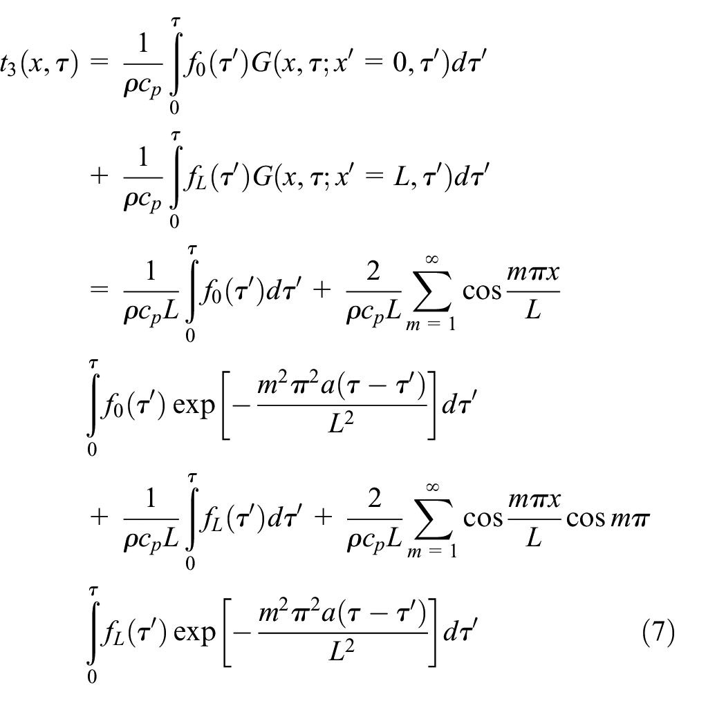
\begin{matrix} t_{3} (x, τ) & = \frac{1}{ρ c_{p}} \int_{0}^{τ} f_{0} (τ') G (x, τ; x' = 0, τ') d τ' \\ + \frac{1}{ρ c_{p}} \int_{0}^{τ} f_{L} (τ') G (x, τ; x' = L, τ') d τ' \\ = \frac{1}{ρ c_{p} L} \int_{0}^{τ} f_{0} (τ') d τ' + \frac{2}{ρ c_{p} L} \sum_{m = 1}^{\infty} \cos \frac{m π x}{L} \\ \int_{0}^{τ} f_{0} (τ') \exp [- \frac{m^{2} π^{2} a (τ - τ')}{L^{2}}] d τ' \\ + \frac{1}{ρ c_{p} L} \int_{0}^{τ} f_{L} (τ') d τ' + \frac{2}{ρ c_{p} L} \sum_{m = 1}^{\infty} \cos \frac{m π x}{L} \cos m π \\ \int_{0}^{τ} f_{L} (τ') \exp [- \frac{m^{2} π^{2} a (τ - τ')}{L^{2}}] d τ' \end{matrix}

(7)

So, the temperature distribution which is a combination of three parts as commented above can be described as

t (x, τ) = t_{1} + t_{2} + t_{3} = t_{3} (x, τ)

(8)

According to the temperature distribution $t (x, τ)$ , the surface temperature of the wall can be described as follows

\begin{matrix} t (0, τ) & = \frac{1}{ρ c_{p} L} \int_{0}^{τ} f_{0} (τ') d τ' + \frac{2}{ρ c_{p} L} \sum_{m = 1}^{\infty} \\ \int_{0}^{τ} f_{0} (τ') \exp [- \frac{m^{2} π^{2} a (τ - τ')}{L^{2}}] d τ' \\ + \frac{1}{ρ c_{p} L} \int_{0}^{τ} f_{L} (τ') d τ' + \frac{2}{ρ c_{p} L} \sum_{m = 1}^{\infty} \cos m π \\ \int_{0}^{τ} f_{L} (τ') \exp [- \frac{m^{2} π^{2} a (τ - τ')}{L^{2}}] d τ' \end{matrix}

(9)

\begin{matrix} t (L, τ) & = \frac{1}{ρ c_{p} L} \int_{0}^{τ} f_{0} (τ') d τ' + \frac{2}{ρ c_{p} L} \sum_{m = 1}^{\infty} \\ \int_{0}^{τ} \cos m π f_{0} (τ') \exp [- \frac{m^{2} π^{2} a (τ - τ')}{L^{2}}] d τ' \\ + \frac{1}{ρ c_{p} L} \int_{0}^{τ} f_{L} (τ') d τ' + \frac{2}{ρ c_{p} L} \sum_{m = 1}^{\infty} \cos^{2} m π \\ \int_{0}^{τ} f_{L} (τ') \exp [- \frac{m^{2} π^{2} a (τ - τ')}{L^{2}}] d τ' \end{matrix}

(10)

For external building walls, the problem can be simplified as follows

a = \frac{λ}{ρ c_{p}} ~ \frac{2 W / (m K)}{2500 kg / m^{3} \times 1000 J / (kg K)} = 8 \times 10^{- 7} m^{2} / s

(11)

\begin{matrix} \frac{m^{2} π^{2} a (τ - τ')}{L^{2}} ~ \frac{{3.14}^{2} \times 8 \times 10^{- 7}}{{0.2}^{2}} \\ m^{2} (τ - τ') = 2 \times 10^{- 3} m^{2} (τ - τ') \end{matrix}

(12)

\begin{matrix} \int_{0}^{τ} f_{0} (τ') \exp [- \frac{m^{2} τ^{2} a (τ - τ')}{L^{2}}] d τ' \\ ~ \int_{0}^{τ} f_{0} (τ') e^{- 2 \times 10^{- 3} m^{2} (τ - τ')} d τ' \end{matrix}

(13)

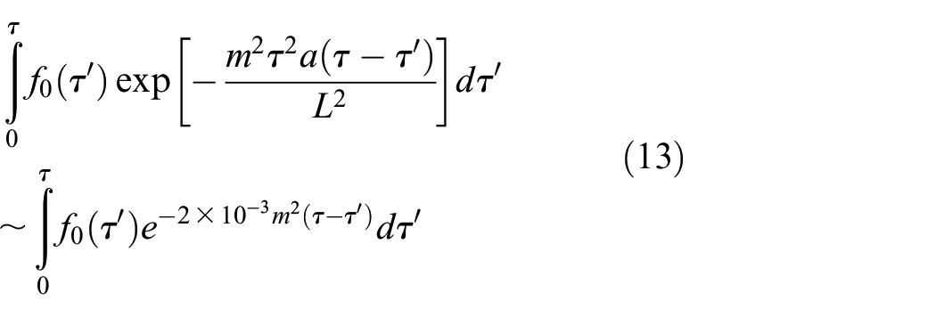
For the integration, we have

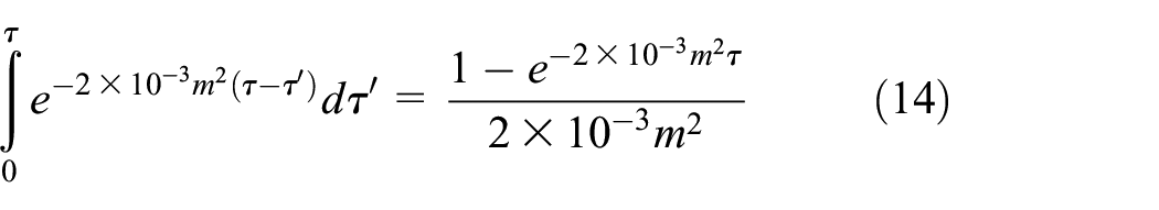
\int_{0}^{τ} e^{- 2 \times 10^{- 3} m^{2} (τ - τ')} d τ' = \frac{1 - e^{- 2 \times 10^{- 3} m^{2} τ}}{2 \times 10^{- 3} m^{2}}

(14)

Considering the integration approximation, $τ_{0}$ can be described as follows when $e^{- 2 \times 10^{- 3} m^{2} τ} = 0.05$

τ_{0} = \frac{\ln 20}{2 \times 10^{- 3} m^{2}} = \frac{1498}{m^{2}} s

When $m = 1$ , $τ_{0} = 1498 s = 25 \min$ ;

When $m = 2$ , $τ_{0} = 6.2 \min$ ;

When $m = 3$ , $τ_{0} = 2.8 \min$ .

The maximum of $τ_{0}$ is 25 min above. However, it is a relatively slower heat transfer process in an actual building, and the boundary heat flux can be regarded as constant during the 25 min. Therefore, equations (9) and (10) can be simplified as follows

\begin{matrix} t (0, τ) = \frac{1}{ρ c_{p} L} \int_{0}^{τ} f_{0} (τ') d τ' + \frac{2}{ρ c_{p} L} f_{0} (τ) \sum_{m = 1}^{\infty} \\ \int_{0}^{τ} \exp [- \frac{m^{2} π^{2} a (τ - τ')}{L^{2}}] d τ' \\ + \frac{1}{ρ c_{p} L} \int_{0}^{τ} f_{L} (τ') d τ' + \frac{2}{ρ c_{p} L} f_{L} (τ) \sum_{m = 1}^{\infty} \cos m π \\ \int_{0}^{τ} \exp [- \frac{m^{2} π^{2} a (τ - τ')}{L^{2}}] d τ' \end{matrix}

(15)

\begin{matrix} t (L, τ) = & \frac{1}{ρ c_{p} L} \int_{0}^{τ} f_{0} (τ') d τ' + \frac{2}{ρ c_{p} L} f_{0} (τ) \sum_{m = 1}^{\infty} \cos m π \\ \int_{0}^{τ} \exp [- \frac{m^{2} π^{2} a (τ - τ')}{L^{2}}] d τ' \\ + \frac{1}{ρ c_{p} L} \int_{0}^{τ} f_{L} (τ') d τ' + \frac{2}{ρ c_{p} L} f_{L} (τ) \sum_{m = 1}^{\infty} \cos^{2} m π \\ \int_{0}^{τ} \exp [- \frac{m^{2} π^{2} a (τ - τ')}{L^{2}}] d τ' \end{matrix}

(16)

The solution of the integration is given as follows

\int_{0}^{τ} \exp [- \frac{m^{2} π^{2} a (τ - τ')}{L^{2}}] d τ' = \frac{L^{2} [1 - \exp (- \frac{m^{2} π^{2} a τ}{L^{2}})]}{m^{2} π^{2} a}

(17)

In the simplified equation, the integration time can be assumed to be infinite $(τ \to \infty)$ , and the solution can be simplified as follows

\int_{0}^{τ} \exp [- \frac{m^{2} π^{2} a (τ - τ')}{L^{2}}] d τ' = \frac{L^{2}}{m^{2} π^{2} a}

(18)

By adding the results of equations mentioned in equations (15) and (16), the solutions of the problem are listed as follows

\begin{matrix} \sum_{m = 1}^{\infty} \int_{0}^{τ} \exp [- \frac{m^{2} π^{2} a (τ - τ')}{L^{2}}] d τ' \\ = \sum_{m = 1}^{\infty} \frac{L^{2}}{m^{2} π^{2} a} = \frac{L^{2}}{π^{2} a} \frac{π^{2}}{6} = \frac{L^{2}}{6 a} \end{matrix}

(19)

\begin{matrix} \sum_{m = 1}^{\infty} \cos m π \int_{0}^{τ} f_{L} (τ') \exp [- \frac{m^{2} π^{2} a (τ - τ')}{L^{2}}] d τ' \\ = \sum_{m = 1}^{\infty} \frac{{(- 1)}^{m} L^{2}}{m^{2} π^{2} a} = - \frac{L^{2}}{12 a} \end{matrix}

(20)

\begin{matrix} \sum_{m = 1}^{\infty} \cos^{2} m π \int_{0}^{τ} \exp [- \frac{m^{2} π^{2} a (τ - τ')}{L^{2}}] d τ' \\ = \sum_{m = 1}^{\infty} \frac{L^{2}}{m^{2} π^{2} a} = \frac{L^{2}}{6 a} \end{matrix}

(21)

Where

\sum_{m = 1}^{\infty} \frac{1}{m^{2}} = \frac{π^{2}}{6}, \sum_{m = 1}^{\infty} \frac{{(- 1)}^{m}}{m^{2}} = - \frac{π^{2}}{12}

(22)

So, according to equations (19)–(22), equations (15) and (16) can be rewritten as follows

\begin{matrix} t (0, τ) & = \frac{1}{ρ c_{p} L} \int_{0}^{τ} [f_{0} (τ') + f_{L} (τ')] d τ' + \frac{2}{ρ c_{p} L} \frac{L^{2}}{6 a} f_{0} (τ) \\ - \frac{2}{ρ c_{p} L} \frac{L^{2}}{12 a} f_{L} (τ) \\ = \frac{1}{ρ c_{p} L} \int_{0}^{τ} [f_{0} (τ') + f_{L} (τ')] d τ' + \frac{L}{6 λ} [2 f_{0} (τ) - f_{L} (τ)] \end{matrix}

(23)

\begin{matrix} t (L, τ) & = \frac{1}{ρ c_{p} L} \int_{0}^{τ} [f_{0} (τ') + f_{L} (τ')] d τ' + \frac{2}{ρ c_{p} L} \frac{L^{2}}{6 a} f_{L} (τ) \\ - \frac{2}{ρ c_{p} L} \frac{L^{2}}{12 a} f_{0} (τ) \\ = \frac{1}{ρ c_{p} L} \int_{0}^{τ} [f_{0} (τ') + f_{L} (τ')] d τ' + \frac{L}{6 λ} [2 f_{L} (τ) - f_{0} (τ)] \end{matrix}

(24)

Because of that the exponent item in Green’s function method before the watch time is relatively little, the surface heat flow function can be regarded as the value at watch time when calculating equations (15) and (16). The integration result of the exponent item is only related to the watch time. Because the value of the watch time is relatively high, the exponent item (18) in the solution can be neglected.

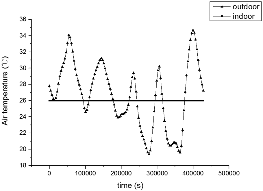
For the usage of real circumstance, we should justify our assumption that the heat flux will not vary significantly within a short amount of time. So verification was performed in three conditions as winter, transition season, and summer testing the heat flux variation in the inner and outer surface of the envelop. Boundary conditions was given as the third kind boundary condition, outdoor temperature was set as the air temperature of winter, spring, and summer in Beijing. Convective heat transfer coefficient was set as 8.7 W/(m² °C) for inner surface and 23 W/(m² °C) for outer surface. Thermal conductivity, density, and specific heat capacity were set as 2 W/(m K), 2500 kg/m³, and 1000 J/(kg K), respectively. Heat flux calculation was performed on a kind of commercial software, scStream, using the finite volume method. The temperature condition and calculation result are illustrated below (Figures 2 –10).

(a) Winter

Temperature condition

Calculation result

(b) Transition season

Temperature condition

Calculation result

Temperature condition

Calculation result

Figure 2.

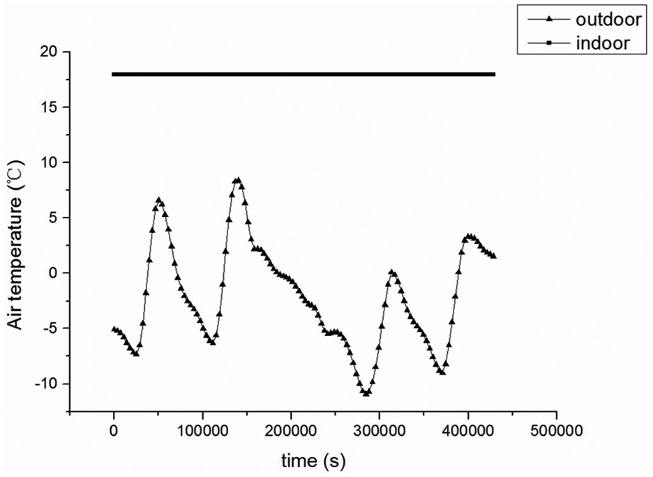
Indoor and outdoor temperature in winter.

Figure 3.

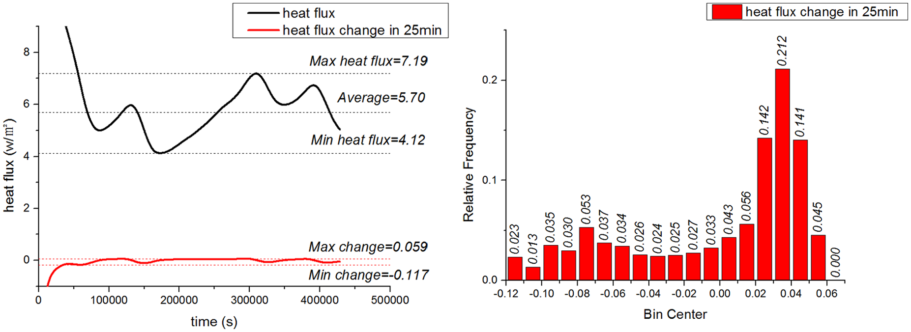
Indoor heat flux and its change in 25 min.

Figure 4.

Outdoor heat flux and its change in 25 min.

Figure 5.

Indoor and outdoor temperature in transition season.

Figure 6.

Indoor heat flux and its change in 25 min.

Figure 7.

Outdoor heat flux and its change in 25 min.

Figure 8.

Indoor and outdoor temperature in summer.

Figure 9.

Indoor heat flux and its change in 25 min.

Figure 10.

Outdoor heat flux and its change in 25 min.

As is shown in the graphs, indoor wall surface has a more slighter fluctuation in the heat transfer process, variation in 25 min is 0.057, 0.078, and 0.067 times of the largest heat flux change in 5 days in winter, transition season, and summer. And for outdoor wall surface, the result is 0.282, 0.345, and 0.400 when variation in 25 min compared with largest heat flux change in 5 days. The range of change in 25 min is large, however, in winter, 83.2% of total time has a change less than ±1 W/m² (the rate is less than 0.088 compared with the largest heat flux change in 5 days). Similarly, for transition season and summer, there are 84.9% and 88.6% of total time and the fluctuation range is less than ±1 W/m² (rate less than 0.101 and 0.116). For most conditions in the practical use, heat flux does not vary significantly within a short amount of time, and the proposed method is valid and accurate.

Extension to double layer building wall

As we know, multilayer envelop is widely used in buildings. For practical application, Green’s function method algorithm for double layer building wall is developed based on the former single-layer working achievements.

Usually, for double layer wall in different materials, there are

\begin{matrix} t_{1} (0, τ) = \frac{1}{ρ_{1} c_{p, 1} L_{1}} \\ \int_{0}^{τ} [f_{0, 1} (τ') + f_{L, 1} (τ')] d τ' + \frac{L_{1}}{6 λ_{1}} [2 f_{0, 1} (τ) - f_{L, 1} (τ)] \end{matrix}

(25)

\begin{matrix} t_{1} (L_{1}, τ) = \frac{1}{ρ_{1} c_{p, 1} L_{1}} \\ \int_{0}^{τ} [f_{0, 1} (τ') + f_{L, 1} (τ')] d τ' + \frac{L_{1}}{6 λ_{1}} [2 f_{L, 1} (τ) - f_{0, 1} (τ)] \end{matrix}

(26)

\begin{matrix} t_{2} (0, τ) = \frac{1}{ρ_{2} c_{p, 2} L_{2}} \\ \int_{0}^{τ} [f_{0, 2} (τ') + f_{L, 2} (τ')] d τ' + \frac{L_{2}}{6 λ_{2}} [2 f_{0, 2} (τ) - f_{L, 2} (τ)] \end{matrix}

(27)

\begin{matrix} t_{2} (L_{2}, τ) = \frac{1}{ρ_{2} c_{p, 2} L_{2}} \\ \int_{0}^{τ} [f_{0, 2} (τ') + f_{L, 2} (τ')] d τ' + \frac{L_{2}}{6 λ_{2}} [2 f_{L, 2} (τ) - f_{0, 2} (τ)] \end{matrix}

(28)

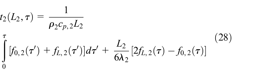
For the junction of the two layers, the temperature and the heat flow of the two layers, it is necessary to establish the following conditions

t_{1} (L_{1}, τ) = t_{2} (0, τ)

(29)

f_{L, 1} = - f_{0, 2}

(30)

From equations (26) and (27), and using the conditions (29) and (30), one obtains

\begin{matrix} t_{1} (L_{1}, τ) = \frac{1}{ρ_{1} c_{p, 1} L_{1}} \\ \int_{0}^{τ} [f_{0, 1} (τ') + f_{L, 1} (τ')] d τ' + \frac{L_{1}}{6 λ_{1}} [2 f_{L, 1} (τ) - f_{0, 1} (τ)] \end{matrix}

(31)

\begin{matrix} t_{1} (L_{1}, τ) = \frac{1}{ρ_{2} c_{p, 2} L_{2}} \\ \int_{0}^{τ} [- f_{L, 1} (τ') + f_{L, 2} (τ')] d τ' + \frac{L_{2}}{6 λ_{2}} [- 2 f_{L, 1} (τ) - f_{L, 2} (τ)] \end{matrix}

(32)

\begin{matrix} \frac{1}{ρ_{1} c_{p, 1} L_{1}} \\ \int_{0}^{τ} [f_{0, 1} (τ') + f_{L, 1} (τ')] d τ' + \frac{L_{1}}{6 λ_{1}} [2 f_{L, 1} (τ) - f_{0, 1} (τ)] \\ = \frac{1}{ρ_{2} c_{p, 2} L_{2}} \\ \int_{0}^{τ} [- f_{L, 1} (τ') + f_{L, 2} (τ')] d τ' + \frac{L_{2}}{6 λ_{2}} [- 2 f_{L, 1} (τ) - f_{L, 2} (τ)] \end{matrix}

(33)

\begin{matrix} (\frac{1}{ρ_{1} c_{p, 1} L_{1}} + \frac{1}{ρ_{2} c_{p, 2} L_{2}}) \int_{0}^{τ} f_{L, 1} (τ') d τ' + (\frac{L_{2}}{3 λ_{2}} + \frac{L_{1}}{3 λ_{1}}) f_{L, 1} (τ) \\ = \frac{1}{ρ_{2} c_{p, 2} L_{2}} \int_{0}^{τ} f_{L, 2} (τ') d τ' + \frac{1}{ρ_{1} c_{p, 1} L_{1}} \\ \int_{0}^{τ} f_{0, 1} (τ') - \frac{L_{2}}{6 λ_{2}} f_{L, 2} (τ) + \frac{L_{1}}{6 λ_{1}} f_{0, 1} (τ) \end{matrix}

(34)

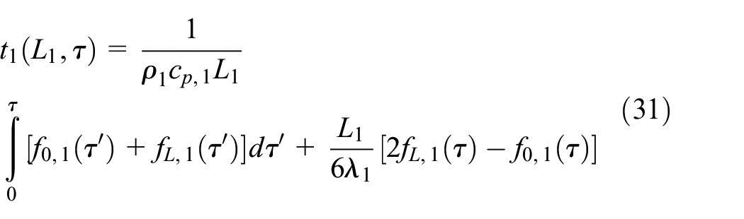
Differentiating this equation with respect to time τ

\begin{matrix} (\frac{1}{ρ_{1} c_{p, 1} L_{1}} + \frac{1}{ρ_{2} c_{p, 2} L_{2}}) f_{L, 1} (τ) + (\frac{L_{2}}{3 λ_{2}} + \frac{L_{1}}{3 λ_{1}}) {f'}_{L, 1} (τ) \\ = \frac{1}{ρ_{2} c_{p, 2} L_{2}} f_{L, 2} (τ) + \frac{1}{ρ_{1} c_{p, 1} L_{1}} f_{0, 1} (τ) \\ - \frac{L_{2}}{6 λ_{2}} {f'}_{L, 2} (τ) + \frac{L_{1}}{6 λ_{1}} {f'}_{0, 1} (τ) \end{matrix}

(35)

\begin{matrix} f_{L, 1} (τ) = \frac{e^{- b}}{\frac{L_{2}}{3 λ_{2}} + \frac{L_{1}}{3 λ_{1}}} \\ \int_{0}^{τ} (\frac{1}{ρ_{2} c_{p, 2} L_{2}} f_{L, 2} (τ') - \frac{1}{ρ_{1} c_{p, 1} L_{1}} f_{0, 1} (τ') - \frac{L_{2}}{6 λ_{2}} {f'}_{L, 2} (τ') + \frac{L_{1}}{6 λ_{1}} {f'}_{0, 1} (τ')) e^{b} d τ' \end{matrix}

(36)

and

\begin{matrix} \int_{0}^{τ} f_{L, 1} (τ') d τ' = \frac{\frac{1}{ρ_{2} c_{p, 2} L_{2}} \int_{0}^{τ} f_{L, 2} (τ') d τ' - \frac{1}{ρ_{1} c_{p, 1} L_{1}} \int_{0}^{τ} f_{0, 1} (τ') - \frac{L_{2}}{6 λ_{2}} f_{L, 2} (τ) + \frac{L_{1}}{6 λ_{1}} f_{0, 1} (τ)}{\frac{1}{ρ_{1} c_{p, 1} L_{1}} + \frac{1}{ρ_{2} c_{p, 2} L_{2}}} - \\ \frac{e^{- b}}{\frac{1}{ρ_{1} c_{p, 1} L_{1}} + \frac{1}{ρ_{2} c_{p, 2} L_{2}}} \int_{0}^{τ} (\frac{1}{ρ_{2} c_{p, 2} L_{2}} f_{L, 2} (τ') - \frac{1}{ρ_{1} c_{p, 1} L_{1}} f_{0, 1} (τ') - \frac{L_{2}}{6 λ_{2}} {f'}_{L, 2} (τ') + \frac{L_{1}}{6 λ_{1}} {f'}_{0, 1} (τ')) e^{b} d τ' \end{matrix}

(37)

in which

b = \frac{\frac{1}{ρ_{1} c_{p, 1} L_{1}} + \frac{1}{ρ_{2} c_{p, 2} L_{2}}}{\frac{L_{2}}{3 λ_{2}} + \frac{L_{1}}{3 λ_{1}}}

(38)

Thus, with the help of equations (37) and (38), the expression of double layer surface temperature can be obtained.

Results and discussion

Simulation model

In order to verify this approximation, the numerical method by MATLAB is introduced to estimate the method error. Four cases under different kinds of boundary conditions are adopted to compare the approximate solutions by Green’s function method, equations (23) and (24), with the exact solutions by the numerical method, equations (9) and (10).

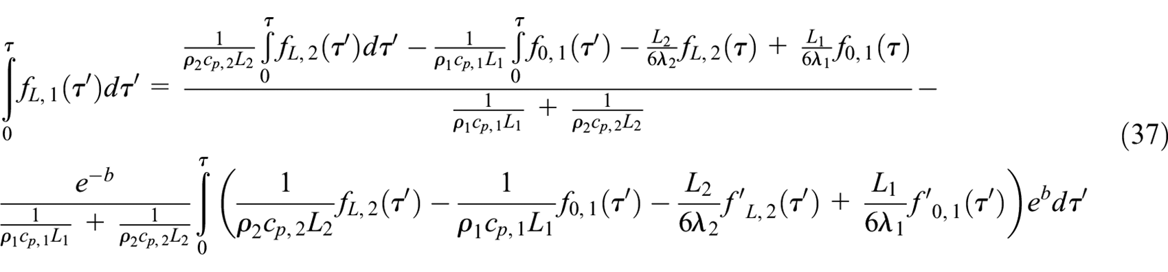
In monolayer conditions (a) to (d), the following parameters of the wall are considered: the thickness $L = 0.2 m$ , the density $ρ = 2500 kg / m^{3}$ , the specific heat capacity $c_{p} = 1000 J / (kg^{\circ} C)$ , and the thermal conductivity coefficient $λ = 2 J / (m K)$ . For double layer wall case, we added another layer in the outer surface, the thickness $L_{2} = 0.1 m$ , the density $ρ_{2} = 1500 kg / m^{3}$ , the specific heat capacity $c_{p 2} = 950 J / (kg^{\circ} C)$ , and the thermal conductivity coefficient $λ_{2} = 1 J / (m K)$ . The results of the heat fluxes of both surfaces and the temperature of the wall are shown in Figure 11(a)–(e).

Figure 11.

a) Heat fluxes of both surfaces of the wall.

Figure 11.

a) Temperature of both surfaces of the wall.

Figure 11.

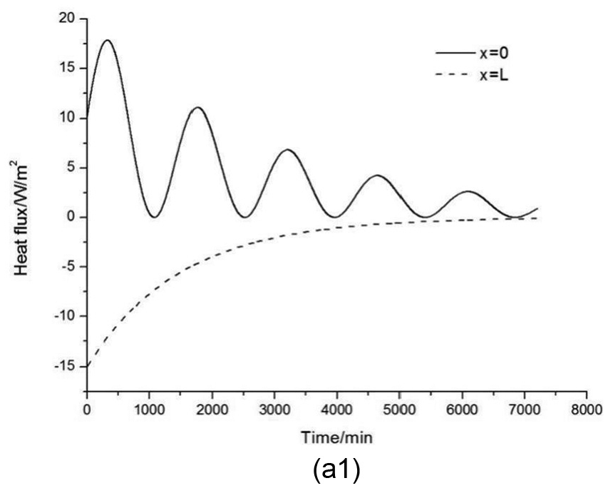
b) Heat fluxes of both surfaces of the wall.

Figure 11.

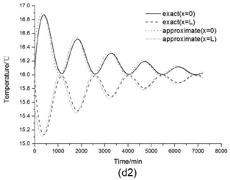
b) Temperature of both surfaces of the wall.

Figure 11.

c) Heat fluxes of both surfaces of the wall.

Figure 11.

c) Temperature of both surfaces of the wall.

Figure 11.

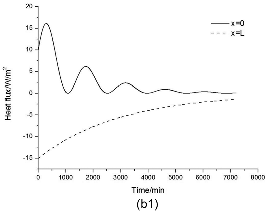
d) Heat fluxes of both surfaces of the wall.

Figure 11.

d) Temperature of both surfaces of the wall.

Figure 11.

e) Heat fluxes of both surfaces of the wall.

Figure 11.

e) Temperature of both surfaces of the wall.

Analysis of simulation results

Monolayer

Boundary condition a

f_{0} = 10 \sin (\frac{2 π}{24 \times 3600} t + 1) e^{- \frac{t}{1.8 \times 10^{5}}} f_{L} = - 15 e^{- \frac{t}{9 \times 10^{4}}}

Solutions

Boundary condition b

f_{0} = 10 \sin (\frac{2 π}{24 \times 3600} t + 1) e^{- \frac{t}{9 \times 10^{4}}} f_{L} = - 15 e^{- \frac{t}{1.8 \times 10^{5}}}

Solutions

Boundary condition c

f_{0} = 10 f_{L} = - 10

Solutions

Boundary condition d

\begin{matrix} f_{0} = 10 \sin (\frac{2 π}{24 \times 3600} t + 1) e^{- \frac{t}{1.8 \times 10^{5}}} \\ f_{L} = - 10 \sin (\frac{2 π}{24 \times 3600} t + 1) e^{- \frac{t}{1.8 \times 10^{5}}} \end{matrix}

Solutions

Double layer

Boundary condition e

\begin{matrix} f_{0} = [10 \times \sin (\frac{10 π}{7200 t}) + 10] \times e^{\frac{- t}{3000}} \\ f_{L} = - [10 \times \sin (\frac{10 π}{7200 t}) + 10] \times e^{\frac{- t}{3000}} \end{matrix}

Solutions

Approximate results by Green’s function are compared with the result of numerical method above.

The results listed in Table 1 for the average relative error in the temperature were calculated as follows

η = \frac{\int_{0}^{t} | T_{approximate} - T_{exact} | dt}{\int_{0}^{t} T_{exact} dt}

(39)

Table 1.

The average relative error of the approximate equation.

Average relative error (%)	Boundary conditions
Average relative error (%)	a	b	c	d	e
x = 0	0.026	0.12	0.12	0.053	0.403
x = L	0.12	0.026	0.12	0.053	0.601

As shown in Table 1, the maximum of the error is only 0.601%. So Green’s function method is verified to be quite effective and accurate. Thus, the original equations can be replaced by the approximate equations. And heat transfer equation of walls can be simplified sharply.

For the last calculation, the double layer wall condition, commercial software scStream was employed. The present new method used 0.184371 s while scStream spend 7 min and 10 s to solve the same problem with 6000 mesh volumes. The time step of Green’s function method is 1 s while the finite volume method (scStream) is 10 s. The new method largely reduced computer run time.

Conclusion

In this article, an analytical solution for dynamic heat transfer problems is presented and Green’s function method is put forward to simplify the heat transfer functions for the solution for the first time. In this method, the function nature and the characteristics of the dynamic heat transfer problem are considered to simplify the method with a highly accelerated calculation. Furthermore, this new method is verified by comparing the approximation solution and the exact solution under four different heat transfer conditions. The analytical solution can be obtained to analyze the building envelope heat performance by applying this method. Furthermore, the double layer building wall analysis model is developed for practical application. It is easy to use and the calculation does not cost much time. So the work in this article is valuable for building design field. Besides, this method has some limits: first, it is not appropriate when the heat flux is high, since the boundary heat flux is simplified to be very low in this model; second, the observation time varies with the building envelope materials. In equation (18), τ is assumed to be infinite. But in the starting of the calculation, especially in the starting 500 s, τ is not so large, so the approximated solution has a relatively large error.

Footnotes

Academic Editor: Takahiro Tsukahara

Declaration of conflicting interests

The author(s) declared no potential conflicts of interest with respect to the research, authorship, and/or publication of this article.

Funding

The author(s) disclosed receipt of the following financial support for the research, authorship, and/or publication of this article: This work is supported by the National Natural Science Foundation of China (Grant No. 51478008) and Beijing Natural Science Foundation (Grant No. 8152007).

References

Nowamooz

Nikoosokhan

Lin

. Finite difference modeling of heat distribution in multilayer soils with time-spatial hydrothermal properties. Renew Energ 2015; 76: 7–15.

Gasparella

Pernigotto

Baratieri

. Thermal dynamic transfer properties of the opaque envelope: analytical and numerical tools for the assessment of the response to summer outdoor conditions. Energ Buildings 2011; 43: 2509–2517.

Oliveti

Arcuri

Mazzeo

. A new parameter for the dynamic analysis of building walls using the harmonic method. Int J Therm Sci 2015; 88: 96–109.

Liu

Zhang

Analysis and evaluation on load of self-conservation wall in harmonic response method. Brick Tile 2011; 7: 9–12.

Wang

Chen

. Applied research of reaction coefficient method for unsteady heat transfer in the wall. Build Environ 2004; 39: 277–280.

Tian

Duan

Niu

. Establishment and experimental validation of a dynamic heat transfer model for concrete radiant cooling slab based on reaction coefficient method. Energ Buildings 2014; 82: 330–340.

Guo

Peng

Liu

Analysis and determination of items amount of reaction coefficient for unsteady heat transfer calculation of wall. J Hunan Inst Sci Technol 2005; 18: 69–72.

Maestrea

Cubillas

Pérez-Lombard

Transient heat conduction in multi-layer walls: an efficient strategy for Laplace’s method. Energ Buildings 2010; 42: 541–546.

Momoniat

McIntyre

Ravindran

Numerical inversion of a Laplace transform solution of a diffusion equation with a mixed derivative term. Appl Math Comput 2009; 209: 222–229.

10.

Lin

Ding

Zhao

. Dynamic model for multi-compartment indirect cooling household refrigerator using Z-transfer function based cabinet model. Int J Therm Sci 2011; 50: 1308–1325.

11.

Kossecka

Kosny

Three-dimensional conduction z-transfer function coefficients determined from the response factors. Energ Buildings 2005; 37: 301–310.

12.

Ruivoa

Ferreirad

Vazc

DC.

On the error of calculation of heat gains through walls by methods using constant decrement factor and time lag values. Energ Buildings 2013; 60: 252–261.

13.

Sala

Urresti

Martín

. Static and dynamic thermal characterisation of a hollow brick wall: tests and numerical analysis. Energ Buildings 2008; 40: 1513–1520.

14.

Haji-Sheikh

de Monte

Beck

JV.

Temperature solutions in thin films using thermal wave Green’s function solution equation. Int J Heat Mass Transf 2013; 62: 78–86.

15.

Ashrafizadeh

Mertiny

McDonald

Determination of temperature distribution within polyurethane substrates during deposition of flame-sprayed aluminum–12 silicon coatings using Green’s function modeling and experiments. Surf Coat Tech 2014; 259: 625–636.

16.

Wang

Tan

KH.

Heat transfer analysis using a Green’s function approach for uniformly insulated steel members subjected to fire. Eng Struct 2005; 27: 1551–1562.

17.

Wang

Z-H

Bou-Zeid

Smith

JA.

A spatially-analytical scheme for surface temperatures and conductive heat fluxes in urban canopy models. Bound: Lay Meteorol 2011; 138: 171–193.

18.

Vasconcellos

CAB

Reis

Mansur

. Experimental validation of numerical solutions using the explicit Green’s approach to simulate transient heat conduction in multilayer systems. Numer Heat Tr A: Appl 2012; 61: 651–668.

A Green’s function solution to the transient heat transfer through the building wall

Abstract

Keywords

Introduction

Formulation of the problem

Extension to double layer building wall

Results and discussion

Simulation model

Analysis of simulation results

Monolayer

Boundary condition a

Boundary condition b

Boundary condition c

Boundary condition d

Double layer

Boundary condition e

Conclusion

Footnotes

Declaration of conflicting interests

Funding

References