
Abstract
In this study, accurate global position system and geographic information system data were employed to reveal multiday routes people used and to study multiday route choice behavior for the same origin–destination trips, from home to work. A new way of thinking about route choice modeling is provided in this study. Travelers are classified into three kinds based on the deviation between actual routes and the shortest travel time paths. Based on the classification, a two-stage route choice process is proposed, in which the first step is to classify the travelers and the second one is to model route choice behavior. After analyzing the characteristics of different types of travelers, an artificial neural network was adopted to classify travelers and model route choice behavior. An empirical study using global position systems data collected in Minneapolis–St Paul metropolitan area was carried out. It finds that most travelers follow the same route during commute trips on successive days. And different types of travelers have a significant difference in route choice property. The modeling results indicate that neural network framework can classify travelers and model route choice well.
Keywords
Introduction
Understanding the multiday route choice behavior of commuters is one of the most important missions in travel behavior modeling. In traditional methods, in order to find the day-to-day differences, respondents were asked to list the used multiday paths. The quality of results is sensitive to the accuracy of respondents’ memories. Global position system (GPS) devices can capture location, speeds, and other information every second. The extensive use of GPS-based travel surveys in the last few years provides an opportunity to trace vehicle movements; hence, GPS will likely become the main mode of travel data collection in the future as smartphone-based platforms for collecting travel data come into use. GPS data present some obvious advantages (and some disadvantages) compared with traditional diary-based surveys. GPS can capture more precise time and location of trip and present less potential for respondents to omit trips from the survey. Particularly, we can easily capture multiple days of travel for each respondent.
If travelers were perfectly rational decision makers, with complete information and perfect computational skills, who cared only about their own travel time, they would choose the shortest paths day by day. 1 However, previous research2,3 has found that fewer than 40% of travelers use the shortest paths, though 90% of subjects took routes that were within 5 min of the shortest paths. Travelers consider criteria beyond travel time,4,5 like monetary cost, 6 avoiding stops, 7 travel time reliability, 8 and aesthetics. 9 In multiday route choice behavior, travelers might want to engage in route search or instead remain on habitual routes. Previous studies show that some commuters do not always follow the same exact route to work, 10 but some do. So we want to differentiate the travelers who usually take a same route and those who do not. Whether travelers switch routes or not may depend on their socio-demographic characteristics, trip and route characteristics, or other circumstances such as weather conditions, time of day, and traffic information. 11
The classification of different route choice analysis models relies on the distinction between different model structures. Some model frameworks were based on artificial intelligence (AI) theory, such as fuzzy logic,12–15 artificial neural networks (ANN),16,17 as well as cognitive psychology.18,19 In the discrete choice framework, multinomial logit (MNL) is the simplest method available, but does not recognize the similarity between routes that share common roadway links. The C-logit, path-size logit (PSL), and path-size correction logit (PSCL) models under this category address this issue by either making changes to the deterministic or the random component of the utility.20–22
Given the importance of multiday route choice modeling and accuracy of GPS data, this study focuses on multiday route choice behavior by evaluating routes followed by residents of the Minneapolis–St Paul metropolitan area, as measured by the GPS component of the 2010 Twin Cities travel behavior inventory (TBI). In the previous study, travelers’ route behavior is analyzed by a sole model.12–22 But as we know, different travelers have different choice decision process. For the first time, in this study, avoiding the uniform analysis of all travelers, travelers are classified into three kinds based on the difference between actual route and shortest travel time path: same route shortest path (SRSP) travelers, same route not shortest path (SRNSP) travelers, and not same route (NSR) travelers. A new way of thinking about route choice modeling, a two-stage route choice process, was proposed. After analyzing the characteristics of different types of travelers, ANN was adopted to classify travelers and model route choice behavior. An empirical study using GPS data collected was carried out in the following section.
The rest of this article is organized as follows: data, methodology, models, empirical result, and conclusion.
Data
Several kinds of data were adopted in this study, including travel data and base data (network and speed data).
The travel data are collected by the GPS component of the 2010 Twin Cities TBI conducted by the Metropolitan Council in the Minneapolis–St Paul metropolitan area. This is detailed in the TBI report for Metropolitan Council and the data available in the Transportation Secure Data Center. Valid data were collected from 278 persons from 250 households as a part of the TBI survey. The data are handled with identification and exclusion steps. The details are shown in Table 1.
TBI GPS trips used/unused for analysis, by reason of exclusion.

GPS: global position system; GIS: geographic information system.
Trips are selected based on mode classification and commute trip identification rules. Mode classification rules are shown in Table 2, while the commute trips are identified based on the location of trip origin and destination. If the distance between a trip origin and house location ranges between 0 and 500 m, and the distance between the destination and work location ranges between 0 and 500 m, the trip is considered as commute trip.
Trips mode classification rules.

The base data include network data and speed data. In the process of data assembly, it requires a high-resolution geographic information system (GIS)-based roadway network for study area. The Lawrence Group (TLG) Twin Cities network is used as base road network in this study, with 290,231 links and 113,864 nodes. It covers the seven-county metropolitan Minneapolis area and is considered by local planners the most accurate GIS street map of the regional network to date. Because in the TLG network, this GIS layer only has information on functional classification and distance of most links in the roadway. It lacks speed information. The speed data source is the TomTom road network data for 2010, which is acquired by the Metropolitan Council for the TBI. TomTom speed data include seven periods in 24-h day. Link travel speed was chosen based on the period of the trip in question’s start time in GPS data.
Once the travel data and base data were assembled, Map Matching was performed. During this process, we identify the specific links of roadway traversed by a vehicle by mapping the points from its GPS trace to an underlying GIS-based roadway network database. In this study, multiday auto commute (H2W) GPS data were matched to TLG Twin Cities network. Then, the actual routes are obtained. The shortest travel time paths are found based on link travel speed on TomTom network. The actual route and shortest travel time path are compared to find their difference. The difference between two actual routes taken on different days is also compared.
Descriptive statistics
Before examining individual’s classification and travel behavior in detail, we report some results of descriptive statistics.
In the sample, 35 travelers had multiple home-to-work trips, averaging 3.11 trips for each traveler, giving 109 trips. Among these multi-trip travelers,
26 of 35 travelers (comprising 83 trips) (or 74%) took the same route each day. Of these
7 of the 26 travelers (or 27%) (comprising 25 trips) took the shortest travel time paths, whom we call SRSP travelers.
19 of the 26 travelers (or 73%) did not generally use the shortest path. These are SRNSP travelers.
9 of 35 travelers (comprising 26 trips) (or 24%) do not take the same route each day, whom we call NSR travelers.
Although the sample is a little small, from this statistic result, we can still find that most travelers (about 75%) choose a same route for their multiday commute trip. Moreover, most of them (about 73%) choose a specific route that is not the shortest travel time route. This shows a similar result with the previous research that most travelers take a same route for commute trip. In the study by Abdel-Aty et al., 10 about 15.5% of the respondents said they use more than one route to work. In our study, about 25% of the traveler might use more than one route. Although this value is a 10% higher than that in the study by Abdel-Aty et al., 10 considering the wide use of information systems, it still can indicate a similar result.
Methodology
Classifier of travelers
Based on the comparison results between routes that are chosen by commuters during their morning commutes, travelers can be divided into two parts: same route (SR) travelers and NSR travelers. SR travelers choose a same route for their commute trips each day, while NSR travelers choose at least two different routes. Furthermore, SR travelers can be classified into two kinds: SRSP travelers and SRNSP travelers. If a traveler is a SRSP traveler, he will choose the shortest travel time path. He is a perfect rational traveler in a sense. SRNSP travelers choose a specific path but not the shortest travel time path. The characteristics of these three kinds of travelers are presented in the following section in detail.
Two-stage choice process
In the models proposed in previous studies, either within the discrete choice modeling framework20–22 or based on other theories, such as AI theory,12–19 all commuters in the sample are analyzed in a same choice model. According to the traveler classification definition, different kinds of travelers have different route choice decision process. Based on this, a two-stage choice process, consisting of a traveler classification stage and a route choice stage, is presented in this study. In the traveler classification stage, drivers are classified into SRSP travelers, SRNSP travelers, or NSR travelers based on some rules or theory. In the route choice stage, each kind of travelers is examined in each way. It is easy to model SRSP travelers because they choose the shortest travel time paths. The result can be output merely based on network topology and link performance disregarding their socio-demographics. For SRNSP and NSR travelers, their route choice behavior can be modeled based on either discrete modeling framework or AI theory. The two-stage choice process framework is presented in Figure 1.

The framework of two-stage choice process.
Neural network classifier
Here, a neural network classifier model is constructed and used to analyze type of travelers as well as SRNSP traveler route choice behavior. Without revealing the mathematical description, a neural network can store vast input–output model mapping. A typical ANN includes three layers: input layer, hidden layer, and output layer. Each layer consists of units (neurons) to represent elements. In the learning phase, the outputs of last layer are feed to the units on the next layers, but there is no feedback to the previous layer. A back propagation (BP) neural network includes signal passing forward and error passing backward. In the error passing backward step, the elements in hidden layers are corrected based on the error assigned to the units. When the error is acceptable or the iteration times reach a number set in advance, the learning phase stops. In the testing phase, the test data are modeling in this classifier. Then, the output of testing phase is compared with the actual valuable. The error is used to estimate the neural network. Figure 2 shows the connection scheme of a typical multi-layer network. In this structure, each input (xi) was assigned an associated weight (wij) to connect input layer and hidden layer, while the connections wjk were assigned to connect hidden layer and output layer. The mathematical formulations of processing functions and error update functions could be found in a lot of previous studies about ANN.16,23–25

A typical multi-layer network.
Models
Property analysis model
As defined in the previous section, travelers are classified into three kinds: SRSP travelers, SRNSP travelers, and NSR travelers. How to analyze and compare properties of different types of travelers? Five variables are proposed in this study.
The following is the formula to describe the overall difference between actual routes (Oaa) taken by one traveler day by day
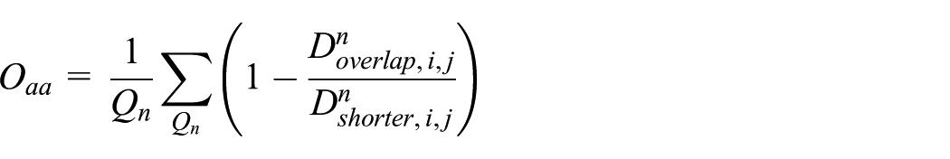
where
For SRSP and SRNSP travelers,
As the description of

where
As we know, the difference between everyday actual route and shortest time route would fluctuate. We also calculated the standard deviation of percentage of overlap
Significances of variables.

Classification model
There are many possible reasons that result in traveler types, including household factors, individual demographic, and employment. We developed a model to classify travelers
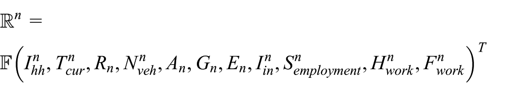
where
The neural network used in this study consists of the input layer, the hidden layer, and the output layer as shown in Figure 3. In our model, three pieces of information, household property, individual socio-demographic, and type of industry, are considered to be important in the traveler classification stage. There are 11 elements in the input layer. They distribute various pieces of information to the network. Driver’s student status can be used as input variable, but it is not considered here because in this study we focus on commute trip. In the above variable, household variables reflect basic socio-economic and demographic characteristics and the degree of familiarity of the transportation network around the neighborhood; individual variables represent the basic information of the travelers, they can reflect the ability of obtaining driver’s previous travel experiences; and industry variables reflect the influence of industry characteristics on the traveler classification.

A three-layer neural network model for traveler classification.
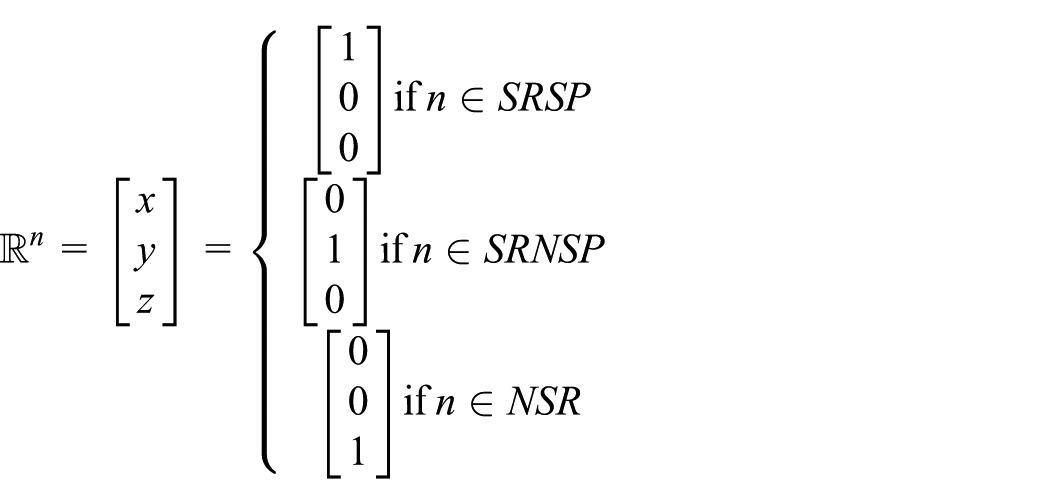
A single processing element in the output layer is used to indicate a classification of travelers among SRSP, SRNSP, and NSR travelers. In previous studies, the testing or prediction results are set as continuous variables. 16 Although it might increase the output hit ratio in the test, it is not an accurate result. In the study, during the training of the neural network, the desired output is set to be a single column matrix with three elements. If a traveler is classified as SRSP traveler, the first element is set to be 1, while others are set to be 0. In the same way, the matrix of SRNSP and NSR travelers can also be set.
Route choice model
For SRSP travelers, they choose the shortest travel time path day by day, so it is easy to build their route choice model as follows

For SRNSP travelers, they choose a same route but not the shortest travel time path. This decision-making behavior is influenced by a multitude of factors, including individual socio-demographic characters, household property, and parameter of route alternatives. Like the traveler classification model, a route choice analysis model based on neural network is proposed for SRNSP travelers. The input valuables of individual socio-demographic and household property are the same as that in neural network model for traveler classification. The third piece of information considered in the route choice decision involves road network topology. The additional input variables to the model are defined as follows:
Distance: weighted distance of routes;
Circuity: weighted ratio of length of route to the Euclidean distance;
Length of longest stretch of roadway (LLSR): weighted ratio of the length longest (distance units) stretch of roadway without intersection to the length of route;
Freeway distance share: weighted ratio of distance traveled on the freeway to the length of route;
Freeway access share: weighted ratio of the travel distance from each trip’s origin to the freeway entrance along the trip to the length of route, ranging from 0 to 1. When it is equal to 1, it means there are no freeway segments included in the route;
Intersection: weighted numbers of intersections;
Left turns: weighted numbers of left turns.
Like the socio-demographic variables, there are also other network variables playing in this, for instance, the location of signals, crash data, or toll. Undoubtedly, these variables might be significant for route choice decision-making behavior, but they were not available in this analysis for information collecting problems. On the other hand, in our model, we added other three variables: (1) the ratio of the length longest (distance units) stretch of roadway without intersection to the length of route (LLSR), (2) the numbers of intersections, and (3) the numbers of left turns. These variables might partly reflect the influence of signals because the influences of them on route choice behavior are all related to less stops or deceleration. The neural network used is shown in Figure 4.

A three-layer neural network model for route choice analysis of SRNSP travelers.
For NSR travelers, they choose at least two routes, this choice decision making is influenced by a lot of factors besides traveler characteristics and network topology, such as weather 26 and incidents. These kinds of variables are not easy to get. They are not included in the collected data in this study. Furthermore, the proportion of this kind of travelers who do not always follow the same exact route to work is very low, 10 this indicates that to some extent, the traffic flow generated by these commuters is much smaller than that generated by travelers who select a same route. And the traffic flow generated by NSR travelers is distributed on the road network randomly, while it is relatively determined for SR travelers. Given these discussions, the route choice analysis of NSR is not considered in this study.
Results
In this study, GPS data collected in Minneapolis–St Paul Metropolitan area are applied to methodology and models proposed in previous sections. The data processing is provided in section “Data.” The property analysis results and neural network analysis results are as follows.
Property analysis results
In model construction phase, five kinds of variables are calculated to describe the property of different kinds of travelers. Using the data provided in this study, a sequence of results is shown in Figure 5. Considering the definition of these variables, from Figure 5 we can find some tendency.

Property analyses of different types of travelers.
It is easy to understand that
Because SRSP travelers choose the shortest travel time path,
The distribution of
From the results, we find that different types of travelers have a significant difference in route choice behavior. It is necessary to analyze a different type of traveler in a different way.
Neural network analysis results
Neural network classifier toolbox in MATLAB is used in this study. And 3 layers and 20 elements in hidden layers are determined in this neural network. In the traveler classification phase, first, 35 travelers are sorted in random order. And the data are divided into two parts: training and testing. In each training cycle, the training vectors are presented to the network in sequential order from traveler 1 to traveler 15, while the remaining travelers are used in testing cycle.
In the route choice analysis phase, the “chosen” route has been identified in the data process step and then other routes that are available to the traveler for making the same trip are determined. This is also called choice-set generation step in discrete modeling framework. Because the set cannot be generated based on the GPS survey data, we construct the choice set by considering the network topology, TomTom data, and locations. To determine a set of alternative route for each origin–destination (OD) pair, enhanced version of the breadth first search link elimination (BFE-LE) was employed. This algorithm has been described in detail in previous research. 27 In contrast with previous studies, here TomTom congested travel time rather than free-flow travel time on links is used as the travel cost. The built-in shortest-path calculation tools from ArcGIS are used. For SRNSP travelers, the choice set consisting of 10 alternatives was generated, including the used route, the shortest travel time path, and other 8 alternatives generated by BFE-LE algorithm. Similar to traveler classification, the routes are sorted in random order, and the last 50 options are set as a testing set, while others are trained in proposed neural network.
Considering the small sample in this study, either in traveler classification or route choice analysis phase, the data are sort in random order 10 times. And the corresponding output is collected. Then, the total output results are compared with the actual event. Tables 4 and 5 present the replication results with respect to traveler classification and route choice decision for the neural network built in the model building phase. Figure 6 shows the neural network training performance. From Tables 4 and 5, we find that 79.09% travelers can be classified in a correct category. The highest error rate happens under the situation that when actual class is NSR, while output class is SRNSP. This can be interpreted that some NSR travelers use a same route in most days during survey period, but choose another one in 1 or 2 days. They are close to SRNSP travelers. Compared with the accuracy rate of traveler classification model, the accuracy rate of route choice analysis model is a little lower; the result is 67.27%. Two errors are nearly equal. In Figure 6, we find the best validation performance is 0.15731 at epoch 16. This indicates that the proposed model has an efficient expression at convergence.
Replication of traveler classification by ANN model.

SRSP: same route shortest path; SRNSP: same route not shortest path; NSR: not same route.
Replication of route choice modeling by ANN model and SWS model.
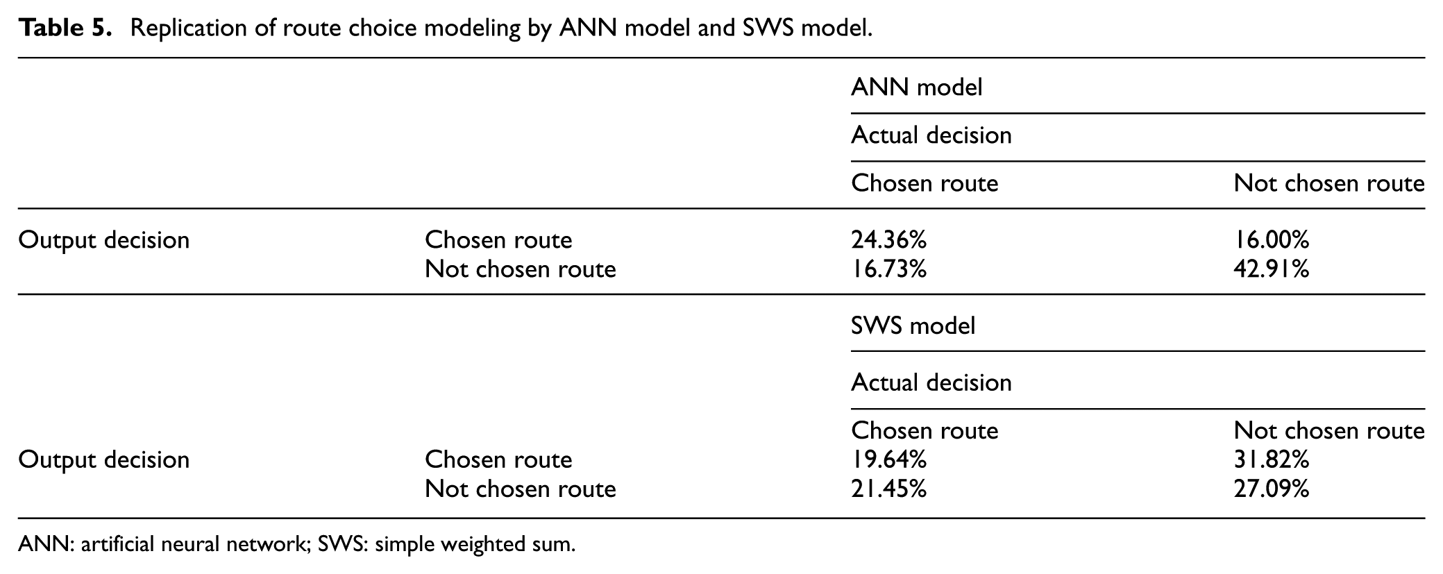
ANN: artificial neural network; SWS: simple weighted sum.

Neural network training performance.
In this study, we use the simple weighted sum (SWS) model as the comparative model to model route choice behavior. In this model, when we set the decision matrix, the influence of route characteristics was assumed to be at a same level with the influence of travel socio-demographic. And moreover, the total influence of household, individual, and industry are all the same. This method requires minimal knowledge of the decision-maker’s priorities and minimal input from decision maker. The equal weights method was popularized and applied in many decision-making problems. 28 The SWS model results are also given in Table 5. Compared with the results of ANN model, we find that, although weighted criteria model used in this study is easier to understand, the accuracy of results is worse than ANN approach. It might be because ANN approach can interpret the influence of factors better than what the comparative model can do for ANN model considering the variables as nonlinear variables, which is much more realistic. Anyway, there might be complex weighted criteria models that can model route choice well, but it is not our research interest in this study.
Conclusion
The study contributes to the literature on traveler classification and route choice behavior analysis literature by analyzing multiday GPS data from the Minneapolis–St Paul region. In previous study, travelers’ route behavior is analyzed by a sole model. But as we know, different travelers have different choice decision process. For the first time, in this study, travelers’ route choice behavior is modeled by classifying the travelers into three types: SRSP travelers, SRNSP travelers, and NSR travelers. And then, each type of travelers is modeled in each way. Besides the classification and route choice models, in order to describe the characteristics of different types of travelers, five variables of each type of travelers are proposed in this study.
Using the GPS data, we find that the descriptive statistics results confirm the result in the previous research. 10 Most travelers choose a same route for commute trip from home to work. From property analysis results, it appears clearly that different types of travelers have different route choice behaviors. They approve that different types of travelers can be modeled in a different way. Traveler classification can be executed before modeling route choice. And then, the traveler classification and route choice behavior are modeled using a neural network. Input layer includes traveler’s demographics (household income, length of time at current address, household region, number of household vehicles, age, gender, education level, type of industry, employment status, number of work hour in 1 week, and flexibility in work hours) and route attributes (distance, circuity, ratio of the length longest stretch, ratio of distance traveled on the freeway, ratio of the travel distance from each trip’s origin to the freeway origin, intersection, and left turns). The testing results of model are acceptable. And compared with SWS model, we find that ANN model can model the route choice behavior better. It might be because ANN model considers the variables as nonlinear variables, which is much more realistic.
Overall, a new way of thinking about route choice modeling is provided in this study. We envision this study as an important contribution toward the development of analyzing traveler’s route choice decision-making process. The results can be further enhanced in other empirical studies with larger hold-out samples.
Footnotes
Acknowledgements
Academic Editor: Hongwei Wu
Declaration of conflicting interests
The author(s) declared no potential conflicts of interest with respect to the research, authorship, and/or publication of this article.
Funding
The author(s) disclosed receipt of the following financial support for the research, authorship, and/or publication of this article: The Federal Highway Administration of the US Department of Transportation is acknowledged for funding the work under a grant to RSG. This research is also supported by the National Natural Science Foundation of China (51178110 and 51378119).