
Abstract
A hybrid method was explored to investigate the generation and near-field radiation of aerodynamic sound from an unsteady turbulent flow over a two-dimensional open cavity and three-dimensional jet flow. A two-dimensional cavity model was established to study the unsteady flow and radiated jet sound. It was revealed that the radiated sound that generated by the boundary layer separation and vortex impact cavity wall intervened in the front of the cavity, and an obvious interference phenomenon appeared. The far-field radiated sound generated by the cavity presented obvious directivity, and the sound pressure in the area located at 45°–135° interval was much higher. Then, the unsteady turbulence jet noises of the elliptical and rectangular nozzles were analyzed. It was revealed that the scale and intensity of the vortexes generated by the elliptical nozzle were larger than those by the rectangular nozzle. The jet noise of the elliptical nozzle is lower than that of the rectangular nozzle. Besides, the sound pressure distributions of the two nozzles presented obvious directivity. The sound pressure in the short-axis direction of the nozzle section was higher than that in the long-axis direction.
Keywords
Introduction
The vortex structure is the main aerodynamic sound source in the flow field. 1 The accuracy of the sound source prediction has great influence on the calculation of the aerodynamic sound. Lighthill 2 was the first to describe the aerodynamic sound source using mathematical method. For some complex flow structures, the calculation of the aerodynamic sound source using the Lighthill stress tensor would be extremely complex and the prediction cost of some engineering noise would become unacceptable. With the rapid development of high-speed computer, some scholars employ the direct numerical simulation (DNS) method to study the jet noise. Freund and colleagues3,4 used the DNS method to simulate the supersonic and subsonic jet noise with the Reynolds number of 2000 and 3600 and the Mach number of 1.92 and 0.9, correspondingly. The simulated flow field data and the total radiated sound pressure level were in good agreement with the experimental results carried out with the same Mach numbers. The superiority of the DNS method in jet noise calculation was fully proved.
The DNS method propounds high-performance computer equipment when used to simulate the high Reynolds number turbulence. Therefore, the “hybrid method” is often used to study the radiated turbulence jet noise.5–8 Its core idea is to calculate the unsteady viscous compressible or incompressible flow first and then to calculate the radiated sound field by the inviscid linear Euler equation (LEE) or the wave equation. It not only greatly reduces the cost of the aerodynamic noise simulation but also makes the far-field acoustic calculation possible. As the calculation cost of the large eddy simulation (LES) method is much smaller than that of the DNS method, it is often adopted in the hybrid method to calculate the unsteady turbulence jet flow and the results are then used to forecast the radiated noise. The studies by Wang and Moin 9 and Zhao et al. 10 showed that the LES method can be used to simulate the low frequency and part of the high-frequency radiated jet noise at high Reynolds numbers with higher accuracy. The process of generation of the jet noise is an unsteady process, while the LES method performs well in the calculation of the unsteady data varying with time. 11 Therefore, the LES method would be the most effective computing tool to study the turbulence jet noise instead of the DNS method in a period of time in the future. 5
Bechara et al. 8 added the extracted sound source term of the turbulence field to the right of the Euler equation to calculate the sound reflection and transmission in the shear flow. Bailly et al. 6 employed a simplified LEE to study the radiated sound flow of two symmetrical rotating vortexes. The method was found to be effective to avoid the growth of the instability wave, and the calculated results were in good agreement with the classical solutions. McMullan et al. 12 applied the LES method to simulate the flow field and obtained the sound source in the near field, then solved the far-field LEE in frequency domain, and next the radiated sound under different jet initial conditions was simulated. The results verified that the method was reliable.
A primary objective of this work was to develop a hybrid method to provide a potential prediction tool for numerical simulation of aerodynamic noise. The LES simulation was used to study the unsteady turbulence field and then the calculation of the sound field was carried out accordingly. The radiated sound in the near field was obtained using the LEE with acoustic source terms. And the Ffowcs Williams and Hawkings (FW-H) equation was used to solve the far-field acoustic. A calculation model was established based on the two-dimensional cavity and the simulation of the unsteady flow, and jet noise was conducted based on the established method. Then, the unsteady turbulence jet noises of the elliptical and rectangular nozzles were analyzed using the developed hybrid method.
Mathematical model
The flow field model
The Reynolds-averaged Navier–Stokes (RANS) turbulence model is operated based on time homogenization model. It is suitable only when the turbulent flow pulsation frequency is lower than the time scale. For the calculation of unsteady turbulent flow with transition process, the RANS turbulence model cannot catch the special flow structure accurately. Usually, the quasi steady-state flow field is calculated using the RANS model, and then the transient flow characteristics are studied by the LES model. Finally, the simulation of aerodynamic sound is carried out according to the simulation results of the LES model. Both the computational cost and the counting period are reduced.
The LES model is a turbulent description method between the DNS method and the Renault time-averaged method. The filter function is adopted to classify the flow structures, and the turbulence is calculated directly by the unsteady Navier–Stokes equation. The sub-grid stress (SGS) model is set up to link large-scale vortexes and small-scale vortexes.
In the LES model, the unsteady Navier–Stokes equations are filtered by the spatial grids, as expressed by the following equations

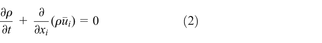
where the variables with over line are the filtered variables,
Equations (1) and (2) are not closed as the SGS stress is unknown. Therefore, the lattice model is established using the related physical quantities to solve the equations. In this article, the Smagorinsky–Lilly lattice model is adopted which supposing the SGS stress to be

where
LEE with source term
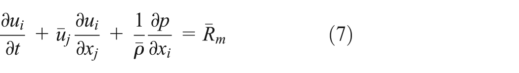
The variables in the flow field can be decomposed into time-averaged terms and fluctuation terms. Then, the variables are inserted in the unsteady Navier–Stokes equation, and the viscosity fluctuation sources are omitted. The following equations can be obtained after rearranging
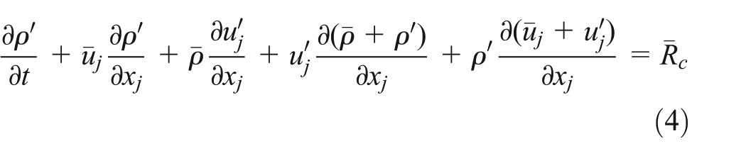

where

The FW-H equation
The volume integrals are dropped and replaced by a so-called permeable FW-H formulation in Fluent. The sound pressure at an observer location, x, can be written as 13

where


Limited boundary truncation technique
In the aerodynamic noise simulation, the accuracy requirements both in space and time should be satisfied. As a fact, the sound wave propagates in free space, while calculation area is limited, and the boundary conditions of fluid field cannot be considered to be far-field free boundary. Hence, the vortexes generated by unsteady flow field shock the boundary and cause large reflection, which would produce “false wave” phenomenon in the flow field. If the “false wave” is greater than the real sound waves in the flow field, the error will be beyond the allowed range. Therefore, special treatment must be taken on the flow calculation boundary of the flow field.
In order to reduce the influence of the outlet boundary on the acoustic calculation, a damp truncation region is set in the front of the outlet boundary of the calculation region. In the damp truncation region, the grids are stretched gradually, as shown in Figure 1. An additional source term is introduced into the control equation of this region to force the transient calculation results to be infinitely close to the corresponding reference value of the quasi steady flow field.

Schematic diagram of the damp truncation region.
The additional source term introduced into the control equation of the damp truncation region is as follows

where
For compressible viscous fluids, the control equations of the damp truncation region are


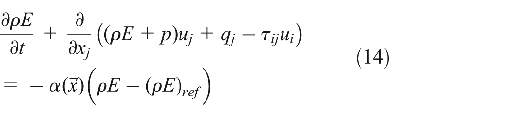
where E is the fluid energy,


where

where
Solution strategy
In order to solve the flow field and aerodynamic noise field, the finite volume method is used to discrete the calculation region, then the unsteady Navier–Stokes equations are solved. The calculated flow results are substituted into the LEE with source item to compute the acoustic pressure field of near field after proper modification. Thereafter, a control surface is set in the flow field and the sound pressure of arbitrary points of far field employing the FW-H equation. The solution strategy is as follows:
The turbulence field is described by RANS model. When the flow field calculation converges stably, the calculated pressure p, velocity
The simulations on the unsteady flow field are carried out using the LES simulation on the basis of the steady flow calculation results. Then, the LEE with source terms is employed to modify the transient simulation results. A program is written using the user-defined function (UDF) to solve the liner Euler equation, and the noise sources of the unsteady flow are determined and the sound pressure propagation of near field can be calculated.
Corresponding control surface is set in the flow field and the calculation time step and the grid number of the control plane are adjusted to guarantee the veracity of the sound field calculation. Then, the FW-H equation is applied to solve the field variables of the control surface and to acquire the sound pressure of arbitrary points of far field. A damp truncation region is arranged in the simulation region, and appropriate source terms are introduced into the control equation of the damp truncation region to reduce the influence of the limited flow field boundary on the noise signal.
Numerical simulation of two-dimensional cavity flow noise
A two-dimensional cavity was taken as the calculation model to conduct the unsteady flow dynamic numerical calculation. The length-to-depth ratio of the cavity was

Schematic of the cavity calculation area.
The whole calculation domain was meshed using quadrilateral grids. The grids had to be fine enough to resolve all the important physics, and the boundary conditions must not affect the solution significantly. In order to verify the grid independence and accuracy, three grid schemes with different grid densities (200 × 200, 300 × 300, and 400 × 400 in the cavity calculation area) were established. The grid node number of the other region was 720 × 460. The sound pressure in the cavity calculation area at different times is shown in Figure 3(a). It can be seen that calculated sound pressure using the three grids was almost the same except only slight changes in pressure amplitude at some times. Figure 3(b) shows the partial enlarged detail during the time of

The sound pressure in the cavity calculation area at different times
A vortex was shed from the cavity front edge and moved to the downstream until it impinged onto the trailing edge of the cavity, generating an acoustic pressure wave, which traveled upstream and led to instabilities in the shear layer and to the shedding of a new vortex. Rossiter 14 developed an empirical formula to predict the resulting oscillation frequencies, which was based on previous studies on edge tones

where f is the frequency, U0 is the velocity of the flow, m is the integer mode number, L is the cavity length, M is the Mach number, 1/kc is the ratio between convection velocity of the vortices and the free-stream velocity, and γ is a factor accounting for the lag time between the passage of a vortex and the emission of a sound pulse at the trailing edge of the cavity. A Fourier analysis of the pressure near the corner of the trailing edge is given in Figure 4. It can be seen that the dominant frequency was obvious. Table 1 shows the comparison of the calculated spectral frequencies and the Rossiter formula. Only the first two modes are shown. The calculation errors were within the acceptable range compared to the results estimated by Rossiter formula.

Fourier analysis of the pressure near the corner of the trailing edge.
Comparison of the calculated spectral frequencies and the estimated results by Rossiter formula.

The cavity unsteady flow field
Figure 5 shows the generation and propagation of the vortexes in the cavity at different times. At

Vorticity at different times: (a)
Radiated acoustic in near field of the cavities
According to the calculated noise source, the sound pressure of the unsteady flow in the cavity was simulated. Figure 6 shows the instantaneous pressure perturbation contours in near field of the cavity. It can be seen that the acoustic wave was corrugated. The shed vortexes moved downstream along with the flow, and radiated acoustic would generate when the vortexes impact the trailing edge of the cavity. The acoustic wave propagated to the upstream and caused the boundary layer to be unsteady. There were strong convection and surface scattering in the front edge of the cavity. The radiated acoustic produced by the boundary layer separation and vortex impact cavity wall intervened, and an obvious interference phenomenon appeared. This was in good agreement with the experimental results carried out by Karamcheti, 15 as shown in Figure 7. Obvious directivity can be seen in the near acoustic field. It was revealed that the radiated acoustic in the area is located at 135°–180° interval and near the front edge of the cavity if taking the z axis to be the rotation axis.

Instantaneous pressure perturbation contours.

Acoustic interference observed in the experiment.
Radiated acoustic in far field of the cavities
In order to analyze the acoustic characteristic in the far field of the cavity, several observation points were set on the arcs of R = 20D and R = 40D with an interval of 15°. The sound pressure level curves of each observation point were obtained by analyzing the detected sound pressure signals, as shown in Figure 8. It can be seen that the sound pressure level of R = 20D was apparently higher than the sound pressure level of R = 40D. It meant that the sound wave attenuated gradually with the increase in the propagation distance. The radiated acoustic in the far field of the cavities also showed obvious directivity as in the near field. The sound pressure in the area located at 45°–135° interval was much higher, and the directivity of the acoustic field had no change with the increase in the observation distance within a certain spread range.

Sound pressure level of different observation angles in far field.
Numerical simulation of the jet noise
The hybrid algorithm was applied to study the effects of nozzle structure on the radiation noise. Two nozzles were designed: an elliptical nozzle and a rectangular nozzle, as shown in Figure 9. The two nozzles were of the same export area and the ratio of long to short half axises of the elliptical nozzle was 1.5:1. Figure 10 shows the grid structure of the model. The model was meshed by the hexahedral grid, and the grids in the nozzle exit and the jet boundary layer whose velocity gradient was great were refined to guarantee high computational accuracy. A damp truncation region was set in the export region near the outlet boundary to reduce the influence of the outlet boundary on the calculation of the sound field. The total grid number was 1,668,864.

The structure of the nozzles.
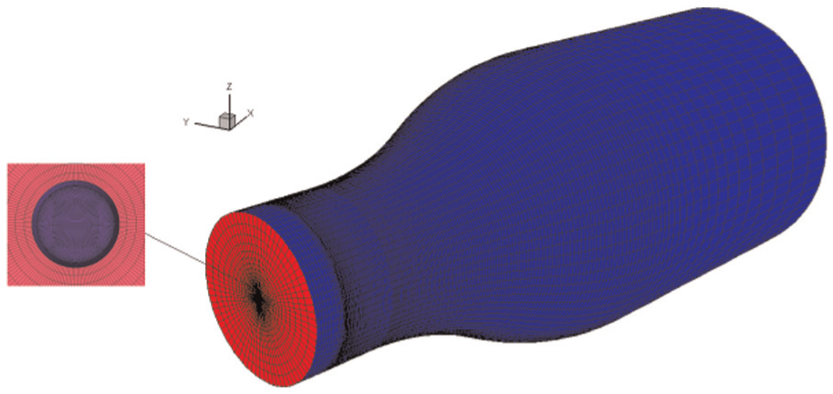
The grid structure of the model.
The calculation region and the boundary conditions of the model are shown in Figure 11. The environment boundary was set to be the pressure outlet. The inlet velocity of the nozzle was 60 m/s and the corresponding Reynolds number was 200,000. The flow temperature and the ambient temperature were both set to be 300 K. The ambient pressure was set to be 101,325 Pa. The impact of air from the environment in the simulation was ignored and the nozzle wall was set to be standard wall condition. Along the axis of the nozzle center, several observation points were set on the arcs of R = 40Dj with an interval of 30°. Besides, the radial section of R = 80Dj at L = 20Dj away from the nozzle exit was set to be monitoring surface.

The schematic of the calculation region.
Analysis of the flow field
When the airflow jet into the environment by the gradual change nozzle, the jet flow intensity attenuated as the strong airflow mixing was generated nearby the border of the jet. Figure 12 shows the velocity distribution of the two different nozzles along the axis of the nozzle center. It can be seen that the flow velocity was maximum near the nozzle exit and the jet was complete turbulence. Comparison of the velocity distribution revealed that the axial velocity of the elliptical nozzle at about L = 8Do away from the nozzle exit showed rapid attenuation which was much higher than that of the rectangular nozzle.

Velocity distribution along the axis of the nozzle center.
When the airflow jet into the environment through the nozzle, large-scale vortexes were formed. In order to have an intuitive understanding of the generation and propagation of the vortexes jet from different nozzles in the turbulent jet flow field, the Q vortex criterion was used to define the vortex structure of the flow field, Q was expressed by

where
Figure 13 shows the iso-surface distribution of
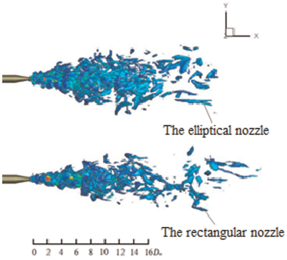
The iso-surface distribution of
Analysis of the sound field
On the basis of the flow field study, the characteristics of the radiated sound were analyzed. Figure 14 shows the sound pressure spectrum curves of the two nozzles in the far field. It can be seen that the sound pressure level of the rectangular nozzle was higher than that of the ellipse nozzle within the entire spectrum. The sound pressure attenuated obviously in the spectrum around 4 kHz. One reason for this was that the small-scale vortexes which would lead to high-frequency sound were ignored in the calculation of the flow field.

The sound pressure spectrum curves of the two nozzles in the far field.
The variation of the nozzle structure not only affected the vortex distribution in the jet field but also affected the characteristics of the radiated sound. Figures 15 and 16 show the sound pressure distributions of the axial cross section and radial section in the far field. It can be seen that the sound pressure of the rectangular nozzle was higher than that of the ellipse nozzle. Combining with the jet flow field analysis results, it can be concluded that the nozzle structure had great influence on the vortex motion and distribution in the jet flow and led to the variation of the jet flow intensity and scope. As revealed in Figure 15, the sound pressure of the observation points in the 30°–65° fan area of the axial cross section at R = 40Dj was little greater than that of the other observation points. Thus, it can be seen that the radiated jet noise was mainly concentrated in the downstream of the jet. Figure 16 shows the sound pressure of the observation points in the radial section of R = 80Dj at L = 20Dj away from the nozzle exit. The sound pressure distributions of the two nozzles presented obvious directivity. And the sound pressure in the short-axis direction of the nozzle section was higher than that in the long-axis direction.

The sound pressure level of the axial cross section at R = 40D.

The sound pressure level in the radial section of R = 80Dj at L = 20Dj away from the nozzle exit.
Conclusion
This article presented a hybrid method to provide a potential prediction tool for numerical simulations of aerodynamic sound problems. The radiated near-field sound was calculated using the LEE with acoustic source terms. The acoustic source terms were extracted from the calculations of the unsteady Navier–Stokes equations using the LES technique. The FW-H equation was adopted to calculate the sound characteristics of the far field. First, the characteristics of the unsteady flow around the cavity had been investigated. The simulation results showed that radiated acoustic was generated along with the formation and breaking of vortexes in the cavity. The radiated acoustic produced by the boundary layer separation and vortex impact cavity wall intervened, and an obvious interference phenomenon appeared. The far-field radiated noise generated by the cavities presented obvious directivity, and the directivity of the acoustic field had no change with the increase in the observation distance within a certain spread range. Then, the hybrid method was used to simulate the unsteady turbulence jet radiated noise of the elliptical and rectangular nozzles. It was revealed that the distribution region, the scale, and intensity of the vortexes generated by the elliptical nozzle in the near field of the nozzle exit were larger than those of the rectangular nozzle. Thus, more ambient fluids were swirled into the jet region for the elliptical nozzle, and the decay rate of the jet velocity was also higher. The sound pressure distributions of the two nozzles presented obvious directivity. The sound pressure in the short-axis direction of the nozzle section was higher than that in the long-axis direction.
Footnotes
Academic Editor: Jiin-Yuh Jang
Declaration of conflicting interests
The author(s) declared no potential conflicts of interest with respect to the research, authorship, and/or publication of this article.
Funding
The authors disclosed receipt of the following financial support for the research, authorship, and/or publication of this article: This research is funded by the National Natural Science Foundation of China (nos 51306166 and 51206101), the Scientific Research Foundation of Shandong Province Outstanding Young Scientist Award (no. BS2013NJ017), the Shandong Province Natural Science Foundation (no. ZR2012EEQ012), and the Qingdao Science and Technology Program of Basic Research Projects (nos. 13-1-4-210-jch and 13-1-4-248-jch).