Adaptive parameters for tracking filters innovation system

Abstract

One of the most important parts in target tracking is the filter algorithm. In the practical engineering, α-β-γ and α-β-γ-δ filters are often applied due to its simpler arithmetic operations. An improved α-β-γ and α-β-γ-δ filters based on parameter identification are proposed to search suitable parameter values at every time step. The tracking errors between the α-β-γ-δ and α-β-γ filters are compared. The results show that the adaptive parameter of the α-β-γ-δ filter exhibits significant improvement in position tracking accuracy over the adaptive parameter of the α-β-γ filter. The simulation results demonstrate that the adaptive parameters of the α-β-γ and α-β-γ-δ filters have better tracking capabilities and good real-time performances.

Introduction

Tracking fast-moving objects, such as air-traffic control, missile interception, and so on, using the discrete-time data to predict the kinematics of a dynamic object is important in military and civilian fields. The α-β tracker is popular because of its simplicity and computationally inexpensive. There have been many derivations for second-order and third-order of the α-β-γ filter. ¹ In 2002, an optimal design α-β-γ filter was presented ² in which a constrained parameter optimization problem was formulated with α, β, and γ being bounded to stay within the stability volume. Lin and Chang ³ have applied them with mathematical models in many researches. Lee et al. ⁴ presented a searching method for the parameter optimization of the third-order α-β-γ filter. Han et al. ⁵ used calculation formula for correlation characteristic of innovation sequence outputted by α-β-γ filter is derived. A correction α-β-γ filtering algorithm is proposed to apply to the simulation of multiple targets. ⁶ The implementation of α-β-γ filter applied in measurement of carrier Doppler is discussed by Jia et al. ⁷

Wu et al.^8–10 presented an optimal design of α-β-γ-δ filter to compare the tracking error between the α-β-γ filter and the α-β-γ-δ filter. As a result, the α-β-γ-δ filter exhibits significant improvement in position tracking accuracy over the α-β-γ filter but at the expense of computational time in search of the optimal filter. To reduce the computation time, the optimization technique via Taguchi’s method, evolution programming (EP), and genetic algorithm (GA) is introduced. These optimal designs of α-β-γ-δ filter and α-β-γ filter are used in the same smoothing parameters for the entire trajectory to minimize tracking position errors. In this article, the author presents a searching method for adaptive parameters of the α-β-γ filter according to the absolute value of the acceleration error and for adaptive parameters of the α-β-γ-δ filter according to the absolute value of the jerk acceleration error at every time step.

Derivation of the α-β-γ and α-β-γ-δ filters

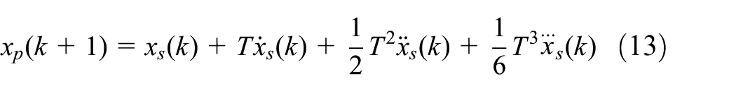
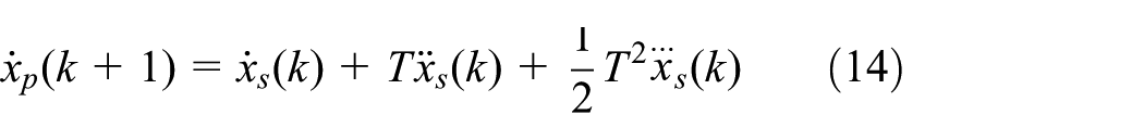
The third-order α-β-γ filter produces smoothing estimates for the next position and velocity of the object based on the current ones. The formulas of α-β-γ filter are represented as follows ¹⁰

$$x_s(k)=x_p(k)+\alpha [x_o(k)-x_p(k)]$$

(1)

$${\stackrel{·}{x}}_s(k)={\stackrel{·}{x}}_p(k)+\frac{\beta }{T}[x_o(k)-x_p(k)]$$

(2)

$${\stackrel{··}{x}}_s(k)={\stackrel{··}{x}}_s(k-1)+\frac{\gamma }{2T^2}[x_o(k)-x_p(k)]$$

(3)

$$x_p(k+1)=x_s(k)+T{\stackrel{·}{x}}_s(k)+\frac{1}{2}{T}^2{\stackrel{··}{x}}_s(k)$$

(4)

$${\stackrel{·}{x}}_p(k+1)={\stackrel{·}{x}}_s(k)+T{\stackrel{··}{x}}_s(k)$$

(5)

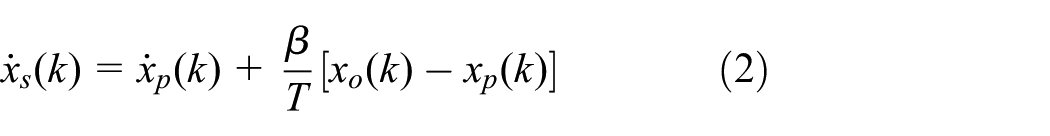
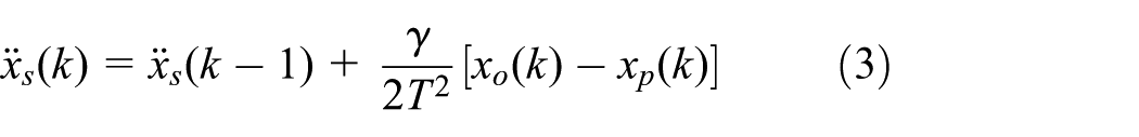
where T is the time step or the time increment, and $x_s,{\stackrel{·}{x}}_s=v_s,{\stackrel{··}{x}}_s=a_s$ are the estimated position, velocity, and acceleration, respectively; the subscripts o, p, and s denote the exact value, the predicted, and smoothed state values, respectively.

Jury’s stability test ¹¹ yields the constraints on α, β, and γ parameters for the α-β-γ filter as shown below

$$0<\alpha <2$$

(6)

$$0<\beta <4-2\alpha$$

(7)

$$0<\gamma <\frac{4\alpha \beta }{2-\alpha }$$

(8)

The fourth-order α-β-γ-δ filter intended for predicting the acceleration is given by

$$x_s(k)=x_p(k)+\alpha [x_o(k)-x_p(k)]$$

(9)

$${\stackrel{·}{x}}_s(k)={\stackrel{·}{x}}_p(k)+\frac{\beta }{T}[x_o(k)-x_p(k)]$$

(10)

$${\stackrel{··}{x}}_s(k)={\stackrel{··}{x}}_p(k)+\frac{\gamma }{2T^2}[x_o(k)-x_p(k)]$$

(11)

$${\stackrel{\dots }{x}}_s(k)={\stackrel{\dots }{x}}_s(k-1)+\frac{\delta }{6T^3}[x_o(k)-x_p(k)]$$

(12)

$$x_p(k+1)=x_s(k)+T{\stackrel{·}{x}}_s(k)+\frac{1}{2}{T}^2{\stackrel{··}{x}}_s(k)+\frac{1}{6}{T}^3{\stackrel{\dots }{x}}_s(k)$$

(13)

$${\stackrel{·}{x}}_p(k+1)={\stackrel{·}{x}}_s(k)+T{\stackrel{··}{x}}_s(k)+\frac{1}{2}{T}^2{\stackrel{\dots }{x}}_s(k)$$

(14)

$${\stackrel{··}{x}}_p(k+1)={\stackrel{··}{x}}_s(k)+T{\stackrel{\dots }{x}}_s(k)$$

(15)

The symbols $x_s,{\stackrel{·}{x}}_s=v_s,{\stackrel{··}{x}}_s=a_s,{\stackrel{\dots }{x}}_s=j_s$ are the estimated position, velocity, acceleration, and jerk, respectively. Jury’s stability test yields the constraints on the β, γ, and δ parameters as follows

$$0<\alpha <2$$

(16)

$$0<\beta <\frac{13}{6}(4-2\alpha )$$

(17)

$$0<\gamma <\frac{4\alpha \beta }{(2-\alpha )}$$

(18)

$$0<\delta <24(2-\alpha )$$

(19)

Optimal design of the α-β-γ and α-β-γ-δ filters

In this study, a searching method for adaptive parameter was applied to optimal design of the α-β-γ and α-β-γ-δ filters.

Each of the three control factors (i.e. α, β, and γ) has four levels of the α-β-γ filter. Thus, there are a total of 64 simulation runs based on full-factorial design.

The four levels are used in equations (1)–(3)

$$\begin{array}{c}\multicolumn{1}{c}{\alpha :[{\alpha }_1,{\alpha }_2,{\alpha }_3,{\alpha }_4]=[0.1,0.7,1.3,1.9]}\\ \multicolumn{1}{c}{\beta :[{\beta }_1,{\beta }_2,{\beta }_3,{\beta }_4]=[4-2{\alpha }_1,4-2{\alpha }_2,4-2{\alpha }_3,4-2{\alpha }_4]}\\ \multicolumn{1}{c}{\gamma :[{\gamma }_1,{\gamma }_2,{\gamma }_3,{\gamma }_4]=[\frac{4{\alpha }_1{\beta }_1}{2-{\alpha }_1},\frac{4{\alpha }_2{\beta }_2}{2-{\alpha }_2},\frac{4{\alpha }_3{\beta }_3}{2-{\alpha }_3},\frac{4{\alpha }_4{\beta }_4}{2-{\alpha }_4}]}\end{array}$$

The α-β-γ filter has 4³ computational runs to compute as equations (1)–(5), and the adaptive parameters are shown below

When i = 1–4

$$\begin{array}{c}\multicolumn{1}{c}{\alpha :[{\alpha }_1,{\alpha }_2,{\alpha }_3,{\alpha }_4]=[0.1,0.7,1.3,1.9]}\\ \multicolumn{1}{c}{\Delta {\beta }_i={\beta }_i-0.1,\Delta {\gamma }_i={\gamma }_i-0.1}\\ \multicolumn{1}{c}{\beta :[0.1,\frac{\Delta {\beta }_i}{3},2·\frac{\Delta {\beta }_i}{3},{\beta }_i]}\\ \multicolumn{1}{c}{\gamma :[0.1,\frac{\Delta {\gamma }_i}{3},2·\frac{\Delta {\gamma }_i}{3},{\gamma }_i]}\end{array}$$

The optimal design is to minimize the absolute value of the acceleration error $|{\stackrel{··}{x}}_s(k)-{\stackrel{··}{x}}_o(k)|$ to find the optimal parameter $({\alpha }^{*},{\beta }^{*},{\gamma }^{*})$ at every time step. The absolute value of the acceleration error is a function of α, β, and γ. First, we give the same parameters β* and γ*. Then, we use a three-point $({\alpha }^1,{\alpha }^{*},{\alpha }^2)$ curve fitting to find the local optimal parameter $\hat{\alpha }$ ; ${\alpha }^1$ and ${\alpha }^2$ are the neighboring levels at the ${\alpha }^{*}$ parameter

$$\begin{array}{c}\multicolumn{1}{c}{f({\alpha }^1,{\beta }^{*},{\gamma }^{*})={\lambda }_{1·}·{\alpha }^1·{\alpha }^1+{\lambda }_{2·}·{\alpha }^1+{\lambda }_3}\\ \multicolumn{1}{c}{f({\alpha }^{*},{\beta }^{*},{\gamma }^{*})={\lambda }_{1·}·{\alpha }^{*}·{\alpha }^{*}+{\lambda }_{2·}·{\alpha }^{*}+{\lambda }_3}\\ \multicolumn{1}{c}{f({\alpha }^2,{\beta }^{*},{\gamma }^{*})={\lambda }_{1·}·{\alpha }^2·{\alpha }^2+{\lambda }_{2·}·{\alpha }^2+{\lambda }_3}\end{array}$$

When the following two conditions are satisfied, we can get the local optimal parameter $\hat{\alpha }=(-0.5^{*}{\lambda }_2)/{\lambda }_1$

$$\begin{array}{c}\multicolumn{1}{c}{f({\alpha }^{*},{\beta }^{*},{\gamma }^{*})\le f({\alpha }^1,{\beta }^{*},{\gamma }^{*})}\\ \multicolumn{1}{c}{f({\alpha }^{*},{\beta }^{*},{\gamma }^{*})\le f({\alpha }^2,{\beta }^{*},{\gamma }^{*})}\end{array}$$

Finally, we can use the same method to find $\hat{\beta }$ and $\hat{\gamma }$ .

Each of the four control factors (i.e. α, β, γ and δ) has four levels of the α-β-γ-δ filter. Thus, there are a total of 256 simulation runs based on full-factorial design.

The four levels are used in equations (16)–(19).

$$\begin{array}{c}\multicolumn{1}{c}{\alpha :[{\alpha }_1,{\alpha }_2,{\alpha }_3,{\alpha }_4]=[0.1,0.7,1.3,1.9]}\\ \multicolumn{1}{c}{\beta :[{\beta }_1,{\beta }_2,{\beta }_3,{\beta }_4]}\\ \multicolumn{1}{c}{=[\frac{13}{6}(4-2{\alpha }_1),\frac{13}{6}(4-2{\alpha }_2),\frac{13}{6}(4-2{\alpha }_3),\frac{13}{6}(4-2{\alpha }_4)]}\\ \multicolumn{1}{c}{\gamma :[{\gamma }_1,{\gamma }_2,{\gamma }_3,{\gamma }_4]=[\frac{4{\alpha }_1{\beta }_1}{2-{\alpha }_1},\frac{4{\alpha }_2{\beta }_2}{2-{\alpha }_2},\frac{4{\alpha }_3{\beta }_3}{2-{\alpha }_3},\frac{4{\alpha }_4{\beta }_4}{2-{\alpha }_4}]}\\ \multicolumn{1}{c}{\delta :[{\delta }_1,{\delta }_2,{\delta }_3,{\delta }_4]}\\ \multicolumn{1}{c}{=[24(2-{\alpha }_1),24(2-{\alpha }_2),24(2-{\alpha }_3),24(2-{\alpha }_4)]}\end{array}$$

The α-β-γ-δ filter has 4⁴ runs to compute as equations (9)–(15), and the adaptive parameters are shown below

$$\begin{array}{c}\multicolumn{1}{c}{\alpha :[{\alpha }_1,{\alpha }_2,{\alpha }_3,{\alpha }_4]=[0.1,0.7,1.3,1.9]}\\ \multicolumn{1}{c}{\Delta {\beta }_i={\beta }_i-0.1,\Delta {\gamma }_i={\gamma }_i-0.1,\Delta {\delta }_i={\delta }_i-0.1}\\ \multicolumn{1}{c}{\beta :[0.1,\frac{\Delta {\beta }_i}{3},2·\frac{\Delta {\beta }_i}{3},{\beta }_i]}\\ \multicolumn{1}{c}{\gamma :[0.1,\frac{\Delta {\gamma }_i}{3},2·\frac{\Delta {\gamma }_i}{3},{\gamma }_i]}\\ \multicolumn{1}{c}{\delta :[0.1,\frac{\Delta {\delta }_i}{3},2·\frac{\Delta {\delta }_i}{3},{\delta }_i]}\end{array}$$

The optimal design is to minimize the absolute value of the jerk error $|{\stackrel{\dots }{x}}_s(k)-{\stackrel{\dots }{x}}_s(k)|$ to find the optimal parameters $({\alpha }^{*},{\beta }^{*},{\gamma }^{*},{\delta }^{*})$ and the local optimal parameters $\hat{\alpha },\hat{\beta },\hat{\gamma },\hat{\delta }$ at every time step.

Numerical simulation

Case 1

It is desirable to compare the tracking errors of the α-β-γ and α-β-γ-δ filters via a numerical simulation process. We consider, for example, the desired signal as a cosine wave

$$y(t)=\cos (t)+\cos (3t)+\cos (5t)$$

In the numerical simulation, with T_start = 0, and T_max = 10, the error in each filter is calculated in different time steps (T = 0.2, 0.1, 0.05, 0.025, 0.125). To track the object, the α-β-γ-δ tracker requires four time steps for initiation, namely

$$\begin{array}{c}\multicolumn{1}{c}{x_p(4)=x_s(4)=x_o(4)}\\ \multicolumn{1}{c}{{\stackrel{·}{x}}_s(4)=\frac{x_o(4)-x_o(3)}{T}}\\ \multicolumn{1}{c}{{\stackrel{··}{x}}_s(4)=\frac{x_o(4)-2x_o(3)+x_o(2)}{T^2}}\\ \multicolumn{1}{c}{{\stackrel{\dots }{x}}_s(4)=\frac{x_o(4)-3x_o(3)+3x_o(2)-x_o(1)}{T^3}}\end{array}$$

In comparison, the α-β-γ tracker requires only three time steps for initiation

$$\begin{array}{c}\multicolumn{1}{c}{x_p(3)=x_s(3)=x_o(3)}\\ \multicolumn{1}{c}{{\stackrel{·}{x}}_s(3)=\frac{x_o(3)-x_o(2)}{T}}\\ \multicolumn{1}{c}{{\stackrel{··}{x}}_s(3)=\frac{x_o(3)-2x_o(2)+x_o(1)}{T^2}}\end{array}$$

The position errors of $L_2$ and $L_{max}$ are defined as

$$\begin{array}{c}\multicolumn{1}{c}{L_2=\frac{\sqrt{\sum _{i=1}^n{(x_p(i)-x_o(i))}^2}}{n}}\\ \multicolumn{1}{c}{L_{max}=max|x_p(i)-x_o(i)|,i=1~n}\end{array}$$

Figures 1–4 show the position, velocity, acceleration, and jerk tracking plot at T = 0.05 for the α-β-γ and α-β-γ-δ filters, respectively. Figures 5–8 estimated that α, β, γ, and δ parameters vary with time plot at T = 0.05 for the α-β-γ and α-β-γ-δ filters.

Figure 1.

Position tracking plot at T = 0.05 for the α-β-γ filter and α-β-γ-δ filter for case 1.

Figure 2.

Velocity tracking plot at T = 0.05 with the α-β-γ filter and α-β-γ-δ filter for case 1.

Figure 3.

Acceleration tracking plot at T = 0.05 for the α-β-γ filter and α-β-γ-δ filter for case 1.

Figure 4.

Jerk tracking plot at T = 0.05 for the α-β-γ-δ filter for case 1.

Figure 5.

Estimated α parameter varies with time at T = 0.05 for the α-β-γ filter and α-β-γ-δ filter for case 1.

Figure 6.

Estimated β parameter varies with time at T = 0.05 for the α-β-γ filter and α-β-γ-δ filter for case 1.

Figure 7.

Estimated γ parameter varies with time at T = 0.05 for the α-β-γ filter and α-β-γ-δ filter for case 1.

Figure 8.

Estimated δ parameter varies with time plot at T = 0.05 for the α-β-γ-δ filter for case 1.

The accuracy improvement shown in each table is the use of α-β-γ-δ filter versus the use of α-β-γ filter, based on L₂ and L_max, respectively. Tables 1 and 2 clearly indicate that the α-β-γ-δ filter consistently outperforms the α-β-γ filter for every given time step. The tracking accuracy improves by more than 50% comparisons between the α-β-γ-δ and α-β-γ filters. As expected, the tracking error monotonically decreases with decreased time step. In other words, the tracking accuracy improves as the time step decreases. In other words, the tracking accuracy improves by more than eight times when the time step is reduced by half. In addition to tracking errors, the computational time has also been studied, and the result is shown in Table 3. The computational time listed in this table is the time needed to calculate the two types of errors. The computational time of the α-β-γ-δ filter is more than four times of that of the α-β-γ filter.

Table 1.

Comparisons of tracking position error on L₂ between α-β-γ filter and α-β-γ-δ filter for case 1.

Time step	α-β-γ	α-β-γ-δ	Improvement (%)
T = 0.2	0.1457	0.0725	50.2
T = 0.1	0.0038	0.0015	60.5
T = 0.05	2.4598e–04	6.0875e–05	75.3
T = 0.025	1.7216e–05	2.2105e–06	87.2
T = 0.0125	1.6678e–06	9.1107e–08	94.5

Table 2.

Comparisons of tracking position error on L_max between α-β-γ filter and α-β-γ-δ filter for case 1.

Time step	α-β-γ	α-β-γ-δ	Improvement (%)
T = 0.2	2.6138	1.5433	41
T = 0.1	0.1113	0.0351	68.5
T = 0.05	0.0119	0.0033	72.3
T = 0.025	2.2105e–06	1.4383e–04	80.4
T = 0.0125	9.1107e–08	8.6517e–06	91.1

Table 3.

Computational time comparisons between α-β-γ filter and α-β-γ-δ filter for case 1.

Time step	α-β-γ		α-β-γ-δ
	Total time (s)	Time/step (ms)	Total time (s)	Time/step (ms)
T = 0.2	0.099	1.998	0.231	4.62
T = 0.1	0.135	1.35	0.376	3.764
T = 0.05	0.201	1.008	0.681	3.408
T = 0.025	0.337	0.845	1.215	3.039
T = 0.0125	0.605	0.757	2.309	2.887

Case 2

For the other example, Chen et al. ¹² presented a constant gain filtering algorithm based on the Jerk model, and the simulation result shows that the accuracy of the α-β-γ-δ filter algorithm is higher than that of the α-β-γ filter algorithm. We simulated it with adaptive parameters of the α-β-γ filter and α-β-γ-δ filter. Supposing the track of target is jerk motion, the motion time from 0 to 100 s, the initial conditions are j(0) = 0 m/s³, a(0) = 0 m/s², v(0) = 200 m/s, and x(0) = 1000 m.

The target tracking motion equations are as follows

1. During $20\le t<40s$ , j(t) = 5 m/s³, uniform jerk motion.

2. During $40\le t<60s$ , a(t) = 40 m/s², uniform acceleration motion.

3. During $60\le t<80s$ , j(t) = −5 m/s³, uniform jerk motion.

4. During $80\le t<100s$ , v(t) = 80 m/s, uniform velocity motion.

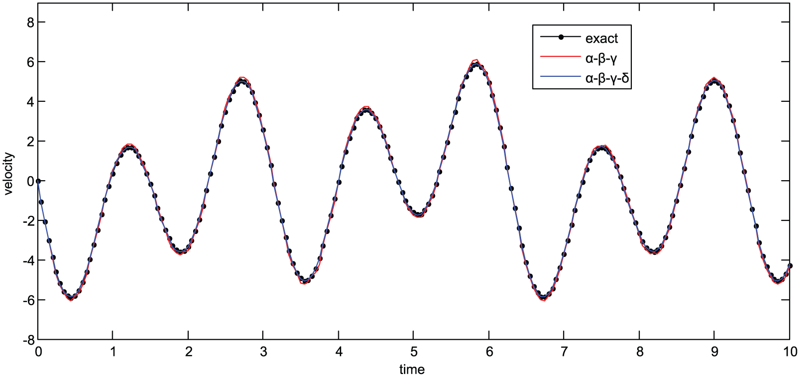
Figures 9–12 show the tracker motion at T = 0.05 with two filters. Tables 4 and 5 summarize the tracking errors on L₂ norm and L_max norm, respectively, from the employment of the α-β-γ and α-β-γ-δ filters at every time step. The average computational time period is 1.5 ms for the α-β-γ-δ filter and 0.4 ms for the α-β-γ filter at every time step (Table 6).

Figure 9.

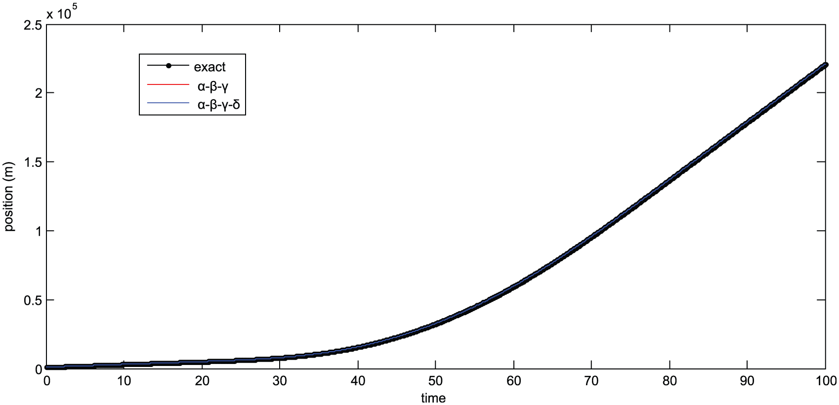
Position tracking plot at T = 0.05 for the α-β-γ filter and α-β-γ-δ filter for case 2.

Figure 10.

Velocity tracking plot at T = 0.05 for the α-β-γ filter and the α-β-γ-δ filter for case 2.

Figure 11.

Acceleration tracking plot at T = 0.05 for the α-β-γ filter and the α-β-γ-δ filter for case 2.

Figure 12.

Jerk tracking plot at T = 0.05 for the α-β-γ-δ filter for case 2.

Table 4.

Comparisons of tracking position error on L₂ between α-β-γ filter and α-β-γ-δ filter for case 2.

Time step	α-β-γ	α-β-γ-δ	Improvement (%)
T = 0.2	6.1253e–04	3.0231e–04	50.6
T = 0.1	5.3232e–05	1.7185e–05	67.7
T = 0.05	4.6146e–06	1.0737e–06	76.7
T = 0.025	4.0382e–07	6.7109e–08	83.4
T = 0.0125	3.5513e–08	4.1943e–09	88.2

Table 5.

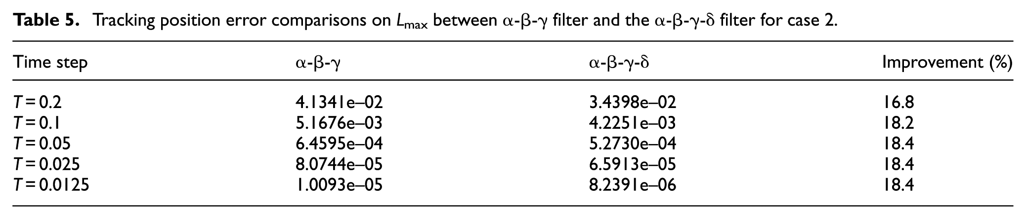
Tracking position error comparisons on L_max between α-β-γ filter and the α-β-γ-δ filter for case 2.

Time step	α-β-γ	α-β-γ-δ	Improvement (%)
T = 0.2	4.1341e–02	3.4398e–02	16.8
T = 0.1	5.1676e–03	4.2251e–03	18.2
T = 0.05	6.4595e–04	5.2730e–04	18.4
T = 0.025	8.0744e–05	6.5913e–05	18.4
T = 0.0125	1.0093e–05	8.2391e–06	18.4

Table 6.

Computational time comparisons between α-β-γ filter and α-β-γ-δ filter for case 2.

Time step	α-β-γ		α-β-γ-δ
	Total time (s)	Time/step (ms)	Total time (s)	Time/step (ms)
T = 0.2	0.030	0.061	0.783	1.56
T = 0.1	0.048	0.048	1.551	1.55
T = 0.05	0.085	0.043	2.999	1.5
T = 0.025	0.157	0.039	6.001	1.5
T = 0.0125	0.307	0.038	11.964	1.5

As shown, the α-β-γ-δ filter outperforms the α-β-γ filter at every time step. Clearly, a fourth-order target tracker of the α-β-γ-δ filter presents a significantly better tracking accuracy than that of the α-β-γ filter.

Conclusion

The simulation results indicate that the optimized α-β-γ and α-β-γ-δ filters based on the adaptive parameters at every time step can provide the approximate position, velocity, and acceleration signals. The α-β-γ-δ filter can simulate jerk signal. The tracking errors between the α-β-γ-δ and α-β-γ filters are compared. The results clearly indicate that the former exhibits a significant improvement in tracking accuracy as compared with the latter. Computation times of both filters are almost lower than the actual physical time, enabling them for applications in real-time control.