Sage Journals: Discover world-class research

Abstract

In this article, a novel artificial neural network integrating feed-forward back-propagation neural network with Gaussian kernel function is proposed for the prediction of compressor performance map. To demonstrate the potential capability of the proposed approach for the typical interpolated and extrapolated predictions, other two classical data-driven modeling methods including feed-forward back-propagation neural network and support vector machine are compared. An assessment is performed and discussed on the sensitivity of different models to the number of training samples (48 training samples, 32 training samples, and 18 training samples). All the results indicate that the proposed neural network in this article has superior prediction performance to the existing feed-forward back-propagation neural network and support vector machine, especially for the extrapolation with small samples. Furthermore, this study can be utilized in refining the existing performance-based modeling for improved simulation analysis, condition monitoring, and fault diagnosis of gas turbine compressor.

Keywords

Compressor performance map prediction feed-forward neural network Gaussian kernel function

Introduction

Compressor behavior which can be represented by performance maps is the main concern for researchers to further understand and improve the design performance of any gas turbine. In the off-design phase, the quality of compressor performance maps is very important for the accuracy of gas turbine performance simulation and diagnostic models. In general, considering the complicated feature of compressor, many experimental studies at various operating and environmental conditions are usually carried out to obtain the performance map of compressor. However, there are only very few experimental data in the full operational range because of the cost and venture of the compressor test. This means that the performance map of a compressor is illustrated as a distribution of discrete points. Besides, fluid flow analysis methodologies including stream line curvature (SLC)¹ method and computational fluid dynamics (CFD) approach² are also used to determine the compressor performance map. But the basic requirement of above two methodologies is that the geometry of the targeted compressor should be known. Therefore, there is a need to developing effective approach to determine the unknown performance parameters of compressor at desired positions.

In the past few decades, various types of prediction methods for compressor performance map have been developed based on the different applications. Moraal and Kolmanovsky³ reviewed the curve fitting methods for centrifugal compressor and turbine characteristics in detail. To solve the problem of lacking experimental data at lower or higher speed conductions, Kurzke⁴ proposed an effective method named auxiliary coordinates (β lines). Sieros et al.⁵ introduced a compressor mapping approach using analytical functions to describe the nonlinear relations between mass flow, pressure ratio, and efficiency. On the basis of Newton–Raphson method, Kim et al.⁶ presented an improved level stacking approach to broaden the application scope of level stacking method. Considering the shape variance of compressor map curves, a new compressor map fitting and modeling method was developed by Tsoutsanis et al.⁷ Besides, Kong et al.⁸ and Li et al.⁹ studied the compressor mapping approaches by means of the scaling and shifting technologies which could improve the fidelity and accuracy of gas turbine models. Although the above approaches have many advantages in the prediction of compressor performance map compromising the characteristic of experimental data and the physical process of compressor component, the nonlinear relationships between different key variable are still inexplicit up to now, which show that the computational accuracy and applicability of these approaches need to be further investigated.

As an effective data-based modeling method, artificial neural network (ANN) is widely used in many areas because of its ability of nonlinear processing and storing massive experimental knowledge.¹⁰ Theoretically, ANN can approximate any nonlinear model and develop the relationships among input and output variables involved in a physical process without considering the underlying physical process.¹¹ Hence, ANN has become increasingly popular for predicting the performance map of compressor in the recent years. Considering the fast convergence characteristics and nonlinear mapping capability of feed-forward back-propagation neural network (BPNN), Feng et al.¹² applied BPNN to predict the characteristic map of compressor working in a low-speed condition. Yu et al.¹³ constructed a three-layer BPNN to overcome the lack of information about stage-by-stage axial-compressor performance. The network was first trained by experiment data, and then its prediction results were regarded as experiment data in the second training. Ghorbanian and Gholamrezaei¹⁴ investigated the applied capability of four kinds of ANN including general regression neural network (GRNN), rotated general regression neural network (RGRNN), radial basis function network (RBFN), and multilayer perceptron network (MLPN) in predicting the compressor performance map in detail. According to their study, it indicated that the RGRNN had the least mean error only for the prediction of interpolation, but MLPN was suggested to provide good prediction for interpolation as well as extrapolation. Besides, Sepehr et al.¹⁵ predicted performance map of rotary vane compressor by BPNN. Their results demonstrated that the statistical performance of BPNN was better than that of nonlinear regression model. Although ANN has been verified to be a very effective method in interpolation prediction of compressor performance map, it is important to point out that a large number of samples are necessary to sufficiently train ANN to get highly prediction accuracy and calculation stability. In order to improve the predicting accuracy of compressor characteristic with small samples (experimental data), different kinds of improved methods have been developed. For example, Kong et al.¹⁶ extrapolated compressor map curve data in the area of off-design by the method of genetic algorithms. Fei et al.¹⁷ proposed a kernel partial least squares (KPLS) model to predict the operating parameters of a centrifugal compressor. Zhao et al.¹⁸ presented a steady-state hybrid modeling of chillers using polynomial neural network compressor model. Tian et al.¹⁹ applied a hybrid artificial neural network—partial least square (ANN-PLS) model to describe the thermodynamic performance of a scroll compressor.

Support vector machine (SVM) is a new machine-learning method in pattern recognition, condition monitoring, and fault diagnosis.^20–22 One of the most important advantages of SVM is a good nonlinear mapping ability with small samples, which largely benefits from the combination of Vapnik–Chervonenki’s theory (VC-theory) and kernel method (kernel tricks).²³ Kernel method is a kind of universal technology which can transform the nonlinear problem into a linear problem through the nuclear space theory.^24,25 Nonlinear vector in low-dimensional space is mapped into high-latitude space by nonlinear function, so the transformed vector in high-latitude space could be treated by linear method. The kernel method, as the core algorithm of SVM, is one of the most influential achievements in machine-learning community.²⁶ There is a member of kernel functions according to Mercer’s theorem of kernel function analysis, such as polynomial kernel function, sigmoid kernel function, and Gaussian kernel function.²⁷ Among these kernel function, Gaussian kernel function had a distinct advantage because of the stronger mapping capability and fewer arguments.^28,29

In this study, a novel network combined BPNN with Gaussian kernel function is proposed to improve the predicting accuracy of compressor performance map. First, compressor performance map and the related problems are introduced. Then, structure and algorithm of the novel network are illustrated after introducing the algorithms of BPNN and SVM. Finally, prediction accuracy and stability of the network are explored when compared with that of BPNN and SVM in the case of a different number of training samples.

Problem description of compressor performance map

Compressor performance map

The characteristic of compressor in the form of Cartesian coordinate’s graph is usually defined as compressor performance map. General speaking, the operating characteristics of compressor can be determined only by two of the four parameters which are corrected speed $(n = n_{c} / T_{in})$ , pressure ratio $(π)$ , corrected flow $(G = G_{c} \sqrt{T_{in}} / p_{in})$ , and the adiabatic compression efficiency of compressor $(η)$ . In practical application, $π$ and $η$ are expressed as a function of the n and G, as shown in equations (1) and (2), respectively

π = f (n, G)

(1)

η = f (n, G)

(2)

Figure 1 shows a performance map of multi-stage axial flow compressor, which only includes speed lines and aerodynamic stability line. Figure 1 is drawn based on experimental data. The original characteristic map of the multi-stage axial compressor, given by the equipment manufacturers, is obtained by compressor characteristic experiment. The coordinate values of six points at each speed line in the original map are extracted to fit the speed lines in Figure 1. In this way, the speed lines in the original characteristic map are reproduced. As shown in Figure 1, it can be seen that there are significance variance between different speed lines, especially at higher n. In other words, π is relative sensitive to the small changes in G with the increase in n. This drawback can cause that the common methods fail to model the compressor maps within a reasonable accuracy.

Figure 1.

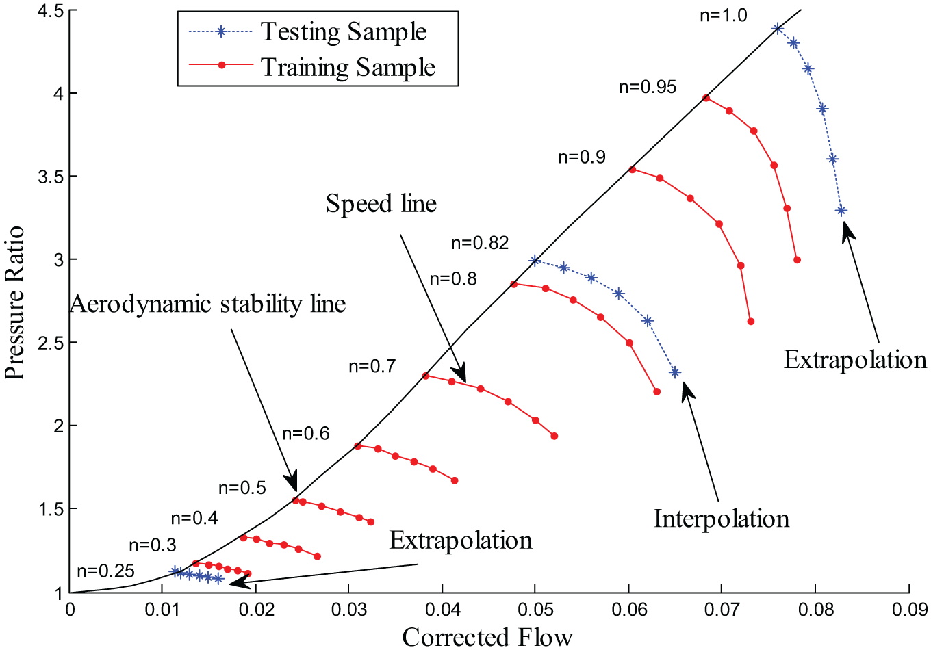
Compressor performance map.

Problem description of interpolation and extrapolation

As previously mentioned, limited experimental data can be obtained in the full operational range considering the cost and venture of compressor test, which means that most of the information (such as the interpolation and extrapolation of data near certain stable state, parameter characteristic of the compressor under start-up or shut-down conduction, and the surge margin of the compressor) need to be predicted. For the interpolated and extrapolated prediction of data, the essential problem is finding the general relation among the mentioned four key variables of compressor. However, the highly nonlinear characteristics of compressor performance are difficult to mathematical model using a small number of experimental data. Therefore, the prediction accuracies of conventional interpolation approaches for compressor performance map are usually unsatisfied. Besides, although ANN can effectively solve the interpolated prediction with higher accuracy, the extension of ANN to extrapolated prediction of compressor performance cure is still debuted and future verified. This is because the prediction accuracy of ANN directly depends on the trained knowledge. And the prediction model based on ANN only develops the potential data relationships among input and output variables, but the physical process is ignored. Therefore, how to utilize the obvious similarity feature between the borders upon speed lines and the nonlinear data analysis advantage of ANN technology to develop a new compressor map fitting and modeling method is significant.

Compared to the prediction of efficiency for compressor map, researches on the prediction of pressure ratio receive more attentions. Therefore, the former is beyond the scope of this study. In other words, the known or input information T is defined as

T = [\begin{matrix} n_{1, 1} & n_{1, 2} & \dots & n_{1, j} & n_{2, 1} & n_{2, 2} & \dots & n_{i, j} \\ G_{1, 1} & G_{1, 2} & \dots & G_{1, j} & G_{2, 1} & G_{2, 2} & \dots & G_{i, j} \end{matrix}]

(3)

where i is the index of speed lines at which the experiment data are selected, so i = 1, 2, …; j is the index of samples selected at each speed line, and j = 1, 2, …; $n_{i, j}$ is corrected speed of the point j at speed line i; and $G_{i, j}$ is corresponding corrected flow of the point.

The target or prediction information Y is determined as in equation (4)

Y = [π_{1}, π_{2}, \dots, π_{q}]

(4)

where q is the total number of target sample.

Feed-forward neural network with Gaussian kernel function

BPNN

As one of the most representative networks of feed-forward neural network, BPNN is composed of simple elementary neuron. The basic principle of an elementary neuron is shown in Figure 2(a). The output of the neuron is expressed in equation (5)

y_{1} = f (\sum_{i = 1}^{k 1} w_{1 i} x_{i} + b_{1})

(5)

where $x_{i}$ is the input variable and $k_{1}$ is the number of inputs. The weight and offset value of the neuron are $w_{1 i}$ and $b_{1}$ , respectively. The output function of the neuron is f, which includes linear transfer function, hyperbolic tangent sigmoid transfer function, and other functions. The output of the neuron is $y_{1}$ .

Figure 2.

Basic principle of BPNN: (a) basic neuron and (b) BPNN.

Figure 2(b) shows the basic structure of BPNN with two inputs and one output. It consists of three layers: one input layer, one hidden layer, and one output layer. The two inputs and one output of BPNN is $x_{a}$ , $x_{b}$ , and $y_{2}$ , respectively. When BPNN is trained according to the learning method of back-propagation algorithm, the weights of neurons between the two adjacent layers are adjusted constantly until the output result matches the target value. Meanwhile, the offset values of neurons are also revised. Therefore, BPNN can map the functional relationship between the inputs and output without knowing its specific expression.

Kernel function

Recently, kernel method is developed to solve the linearly inseparable or nonlinear problems in classification. According to the basic theory of kernel method which is shown in Figure 3, the linearly inseparable data in low-dimensional space (L) can be mapped to a high-latitude space (H) by the nonlinear mapping function $ϕ (x)$ . Then, the mapped data become linearly separable in space (H). The latitude of space H is limited or unlimited.

Figure 3.

The basic principle of kernel theory.

It is worth noting that the kernel function is always expressed as a form of the inner product. So the kernel functions can be applied directly without knowing the specific expression of the nonlinear mapping function, which avoids the problem of solving nonlinear mapping function.

In practical applications, the selection of the appropriate kernel function is vital. Nowadays, there are a lot of different kernel functions according to Mercer’s theorem of kernel function analysis. Three representative kernel functions are listed as follows:

Polynomial kernel function

K (x, y) = {〈 x, y 〉}^{d}

(6)

where $〈 x, y 〉$ denotes the dot product between x and y, and d is a constant parameter.

Sigmoid kernel function

K (x, y) = \tan h (α_{1} 〈 x, y 〉 + α_{2})

(7)

where $α_{1}$ and $α_{2}$ are the constant parameters.

Gaussian kernel function

K (x, y) = \exp (- \frac{{‖ x - y ‖}^{2}}{σ})

(8)

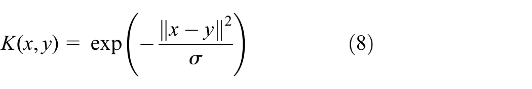
where $σ$ is the constant parameter.

Gaussian kernel function BPNN

A novel neural network combining BPNN and Gaussian kernel function is proposed which can be named as Gaussian kernel function back-propagation neural network (GBPNN). The structure of GBPNN includes one input layer, one Gaussian kernel layer, two hidden layers, and one output layer, as illustrated in Figure 4.

Figure 4.

Algorithm structure of GBPNN.

The two input variables of GBPNN are corrected speed n and corrected flow G, and ratio pressure π is selected as the output variable of GBPNN, so it can match the model of compressor performance map which is shown in equation (1).

The dotted line box in the Gaussian kernel layer is the Gaussian neurons, and its amount is determined by the number of speed lines that obtained the samples, just as it is illustrated in equation (3). The numbers of neurons in the hidden layer and output layer are the same as that of BPNN, which can be determined by optimized algorithm.

K in the dotted line box represents Gaussian kernel function as expressed in equation (8), and the output of Gaussian neurons $T_{Gi}$ is expressed as in equation (9)

T_{Gi} = \exp (- \frac{{‖ n_{i, j} - n_{i} ‖}^{2}}{σ}) \times G_{i, j}

(9)

where $h_{1 k}$ is the output of neuron in hidden layer I and is expressed as in equation (10)

h 1_{k} = f 1 (\sum_{i = 1} w 1_{ki} {T_{G}}_{i} + b 1_{k})

(10)

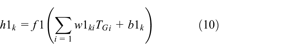
where k is the index of neurons in hidden layer I, $w 1_{ki}$ is the weight between neuron i in Gaussian kernel layer and neuron k in hidden layer I, $b 1_{k}$ is threshold value of the neuron k, and $f 1$ is the transfer function of the neuron k.

Similarly, $h 2_{l}$ in equation (11) represents the output of neuron in hidden layer II

h 2_{l} = f 2 (\sum_{k = 1} w 2_{lk} h 1_{k} + b 2_{l})

(11)

where l is the index of neurons in hidden layer II, $w 2_{lk}$ is the weight between neuron k in hidden layer I and neuron l in hidden layer II, $b 2_{l}$ is threshold value of the neuron l, and $f 2$ represents transfer function of the neuron l.

In equation (12), $h 3_{m}$ represents output of neuron in output layer

h 3_{m} = f 3 (\sum_{l = 1} w 3_{ml} h 2_{l} + b 3_{m})

(12)

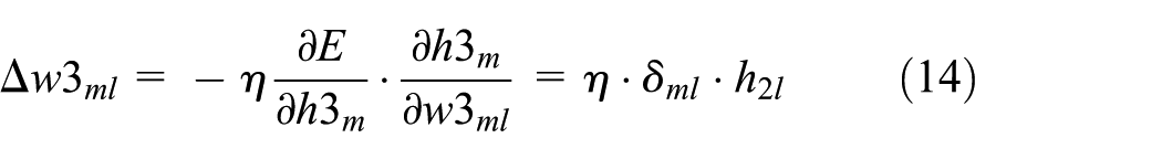
where m is the index of neurons in output layer, $w 3_{ml}$ is the weight between neuron l in hidden layer II and neuron m in output layer, $b 3_{m}$ is threshold value of the neuron m, and $f 3$ denotes transfer function of the neuron m.

The error function is defined as in equation (13)

E = \frac{1}{2} \sum {(π - h_{3 m})}^{2}

(13)

Weight $w 3_{ml}$ is adjusted as in equation (14)

Δ w 3_{ml} = - η \frac{\partial E}{\partial h 3_{m}} \cdot \frac{\partial h 3_{m}}{\partial w 3_{ml}} = η \cdot δ_{ml} \cdot h_{2 l}

(14)

where $η$ is the learning coefficient which usually defined as a constant, $δ_{ml} = (π - h_{3 m}) \cdot f 3'$ , and $f 3'$ is the derivative of $f 3$ .

Threshold $b 3_{m}$ is calculated as shown in equation (15)

Δ b 3_{m} = - η \frac{\partial E}{\partial h 3_{m}} \cdot \frac{\partial h 3_{m}}{\partial b 3_{ml}} = η \cdot δ_{ml}

(15)

Weight $w 2_{lk}$ is adjusted as in equation (16)

Δ w 2_{lk} = - η \frac{\partial E}{\partial h 3_{m}} \cdot \frac{\partial h 3_{m}}{\partial h_{2 l}} \frac{\partial h_{2 l}}{\partial w 2_{lk}} = η \cdot δ_{lk} \cdot h 1_{k}

(16)

where $δ_{lk} = \sum_{l = 1} δ_{ml} \cdot w 3_{ml} \cdot f 2'$ , and $f 2'$ is the derivative of $f 2$ .

Threshold $b 2_{l}$ is adjusted as in equation (17)

Δ b 2_{l} = η \cdot δ_{lk}

(17)

Weight $w 1_{ki}$ is revised as follows

Δ w 1_{ki} = η \cdot δ_{ki} \cdot {T_{G}}_{i}

(18)

where $δ_{ki} = \sum_{k = 1} δ_{lk} \cdot w 2_{lk} \cdot f 1'$ , and $f 1'$ is the derivative of $f 1$ .

Threshold $b 1_{k}$ is adjusted as in equation (19)

Δ b 1_{k} = η \cdot δ_{ki}

(19)

The calculation steps of BPNN

GBPNN method is the combination of BPNN and Gaussian kernel function. It can be seen from Figure 4 that errors are forward passed and weights (threshold) are reversely adjusted in GBPNN, so GBPNN model is a kind of forward network. The calculation steps of GBPNN are the same as most of the other forward neural networks, just as it is shown in following:

Step 1: select training and testing samples;

Step 2: determine parameters of GBPNN;

Step 3: train GBPNN with training samples;

Step 4: stop training if the error is acceptable;

Step 5: predict compressor performance map;

Step 6: analyze prediction accuracy with testing samples.

Results and discussion

In this section, GBPNN proposed in this article will be applied to predict the performance map of a multi-stage axial flow compressor. To demonstrate the potential capability of GBPNN for the interpolation and extrapolation, other two classical data-driven modeling methods named BPNN and SVM are also compared. The three models above are all realized based on M language in the MATLAB simulation environment. Besides, an assessment is performed and discussed on the sensitivity of different models to the number of training samples (48 training samples, 32 training samples, and 18 training samples). Furthermore, the prediction accuracy of GBPNN, BPNN, and SVM is evaluated by the mean absolute error (MAE) which can be calculated using the following functions

MAE = \frac{1}{N} \sum_{v = 1}^{N} | π_{v} - h_{3 mv} |

(20)

where N is the sample number, $π_{v}$ and ${h_{3 m}}_{v}$ are the target value and prediction result, respectively.

Sample partition and data preprocessing

For the prediction of GBPNN, BPNN, and SVM, the data sample is vital. In this study, six known experimental data at every speed line (n = 0.95, n = 0.9, n = 0.8, n = 0.7, n = 0.6, n = 0.5, n = 0.4, and n = 0.3) shown in Figure 1 are selected as training samples according to the sample selection method proposed in Ghorbanian and Gholamrezaei.¹⁴ Therefore, 48 samples can be obtained to train GBPNN, BPNN, and SVM. Similarly, 18 experimental data at speed lines of n = 1.0, n = 0.82, and n = 0.25 (blue dashed line in Figure 1) are selected as the testing samples which are divided into interpolated prediction and extrapolated prediction. In practical, considering the deficiency of experiment data at high- and low-speed conductions, the prediction of samples at corrected speed n = 1.0 is regarded as the extrapolation of high speed, and that of n = 0.25 is defined as extrapolation of low speed. Besides, the prediction of n = 0.82 in the middle of performance map is regarded as interpolation.

To eliminate the influence of the sample dimension, all the samples should be normalized using the following function

s_{k} = \frac{2 (s - s_{\min})}{s_{\max} - s_{\min}} - 1

(21)

where s is the original sample, $s_{k}$ is the normalized sample with range [−1, 1], $s_{\max}$ and $s_{\min}$ are the maximum and minimum of original sample, respectively.

Parameters configuration of prediction models

When the samples are obtained, the structures and related parameters of every prediction model need to be determined. The parameter configurations of BPNN are fully in accordance with that of Ghorbanian and Gholamrezaei.¹⁴ In other words, BPNN consists one input layer, two hidden layers, and one output layer, where the corresponding neuron numbers are 2, 10, 10, and 1, respectively, for the prediction with 48 training samples. According to the basic principle of GBPNN, the number of neurons in Gaussian kernel layer will be determined by the number of speed lines that obtained the training samples. This means that the numbers of neurons in Gaussian kernel layer of GBPNN are 8 for the prediction with 48 training samples. In order to reasonably compare the prediction performance of GBPNN and BPNN, GBPNN also includes the same hidden layers, output layer, and the corresponding neuron numbers of hidden layers and output layer. In other words, the structure of GBPNN is 8-10-10-1. By analyzing the effects of coefficient $σ$ on prediction error in Figure 5, it can be found that the minimum sum of prediction error can be obtained when $σ$ is 0.5. Moreover, for GBPNN and BPNN, hyperbolic tangent sigmoid transfer function and linear transfer function will be used in the hidden layers and output layer, respectively, and Levenberg–Marquardt algorithm is selected as learning method.

Figure 5.

The sum of prediction error with value of gain coefficient in Gaussian kernel function.

Kernel function (ker), non-separable case (C), and loss function (loss) are the very important factors for SVM. In this study, radial basis function is selected as the kernel function (ker = rbf), and radial basis width parameter (p1) and insensitivity (e) are 0.3 and 0.001, respectively. Besides, epsilon insensitive function is taken as the loss function. Non-separable case is 800.

Prediction of compressor performance map with 48 training samples

Both the extrapolated and interpolated predictions are performed in this comparison. The training and testing samples used in different prediction models are same, and the initial weights of GBPNN and BPNN are given randomly.

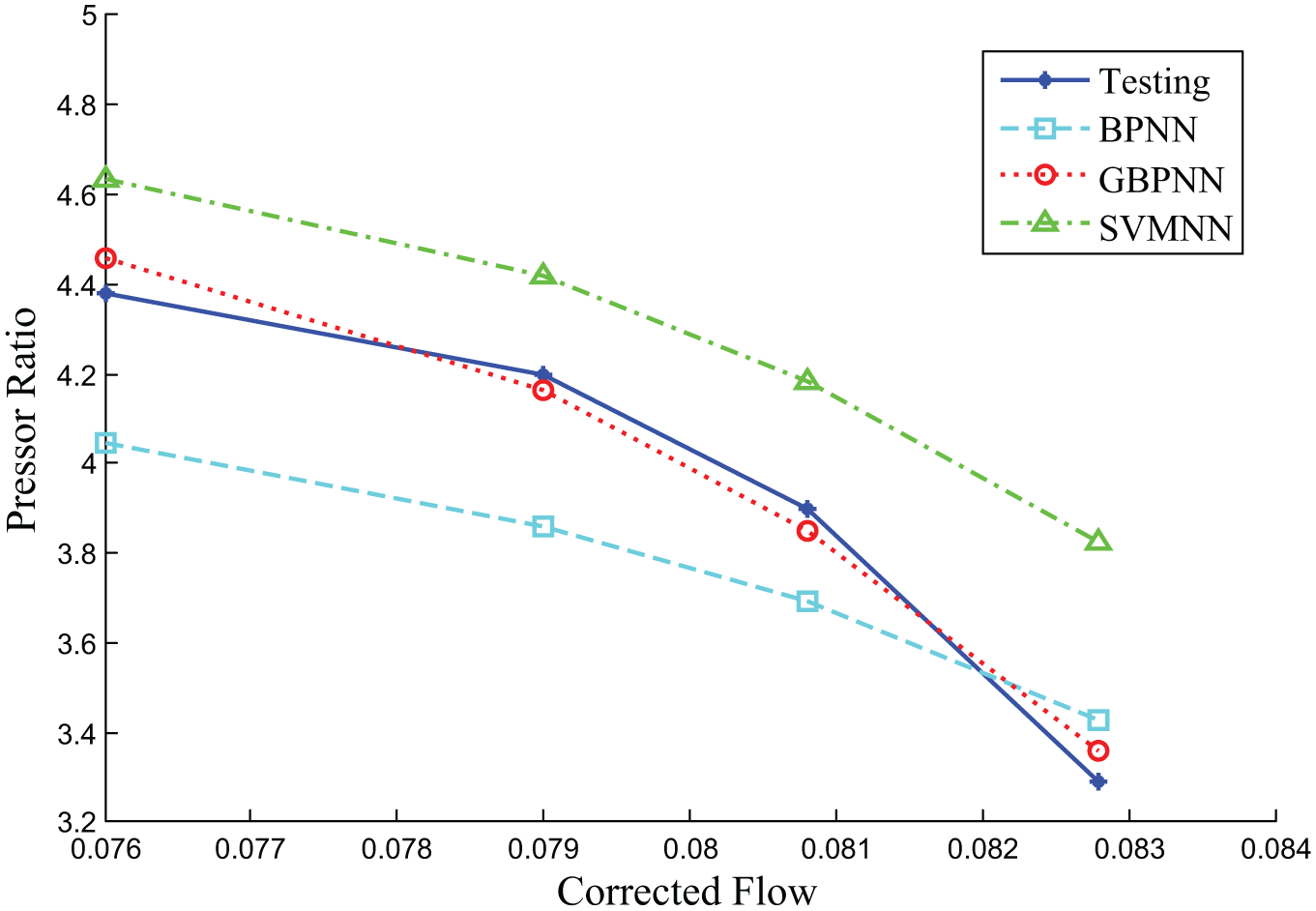
Figure 6 shows the comparison of GBPNN, BPNN, and SVM for the interpolated and extrapolated prediction of compressor performance map. As shown in Figure 6, it can be seen that the values at speed lines of n = 0.82 predicted by every of the above three models are in good agreement with the experimental data, which means that there are perfect prediction accuracy of GBPNN, BPNN and SVM in interpolated prediction. Besides, a careful inspection of Figure 6 reveals that the difference of GBPNN, BPNN, and SVM is obvious when they are used to predict the extrapolation of compressor performance map, especially at n = 1.0. As shown in Figure 7, GBPNN has the best prediction performance, following SVM and BPNN, respectively.

Figure 6.

Prediction of compressor performance with 48 training samples.

Figure 7.

Extrapolation prediction of compressor performance (n = 1.0) with 48 training samples.

To eliminate the influence of randomness of weights and thresholds on GBPNN and BPNN, and avoid the problems of stiffness and blockage in local minima, Figure 8 illustrates the variations of MAE using different models with 50 times prediction. According to the results, it is observed that BPNN has a higher sensitivity than GBPNN to the initial weights and thresholds, which shows that the prediction performance of BPNN is difficult to satisfy the prediction accuracy demand of compressor performance map. Besides, although the outputs of SVM are unchanged because of its fixed parameters, the MAEs of SVM are more than those of GBPNN with 48 training samples. Table 1 shows the mean value of MAE for 50 times. For the GBPNN, the mean value of MAE for 50 times is only 0.014 which is obviously lower than those of SVM (0.025) and BPNN (0.080). All of these demonstrate that GBPNN is superior to BPNN and SVM in accuracy and stability of the prediction of compressor performance map.

Figure 8.

MAE curves of 50 times prediction with 48 training samples.

Table 1.

The mean of MAE of 50 times prediction with three kinds of training samples.

Network	48 samples	32 samples	18 samples
GBPNN	0.014	0.045	0.289
SVM	0.025	0.043	0.250
BPNN	0.080	0.146	1.151

MAE: mean absolute error; GBPNN: Gaussian kernel function back-propagation neural network; SVM: support vector machine; BPNN: back-propagation neural network.

Prediction of compressor performance map with 32 training samples

Considering the fact that the prediction accuracy of data-based modeling approach can be affected by the number of training sample, the prediction performance of GBPNN, BPNN, and SVM needs to be further analyzed. In this study, 30% of the total samples are cut off, which means that only 32 samples (four experimental data at each speed lines of n = 0.95, n = 0.9, n = 0.8, n = 0.7, n = 0.6, n = 0.5, n = 0.4, and n = 0.3) are used to train the above three prediction models. It is noting that all the structures and related parameters of every model are same as those of 48 training samples.

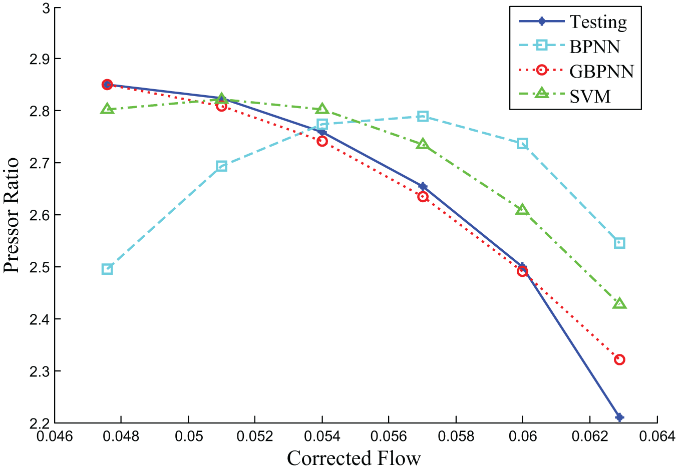
Figure 9 presents the prediction results using GBPNN, BPNN, and SVM with 32 training samples. From the figure, it is easily found that all the prediction accuracies of above three models are acceptable for the interpolation (n = 0.82) of compressor performance map. However, for the extrapolation at speed lines of n = 1.0, only GBPNN has a relatively acceptable prediction accuracy, as shown in Figure 10.

Figure 9.

Prediction of compressor performance with 32 training samples.

Figure 10.

Extrapolation prediction (n = 1.0) of compressor performance with 32 training samples.

The results shown in Figure 11 and Table 1 indicate that all MAEs of GBPNN, BPNN, and SVM are bigger than those of 48 training samples. The mean values of MAE for prediction of 50 times are 0.045 for GBPNN, 0.043 for SVM, and 0.146 for BPNN. This is because the above three prediction models may not be trained well when the training sample is smaller. Besides, BPNN is so sensitive to the number of training samples that its prediction accuracy decreases significantly with the reduction in training sample number. However, GBPNN has a higher steady performance than BPNN because of the addition of Gaussian kernel layer. Moreover, it should be noted that SVM can provide the lowest mean MAE for the prediction of 50 times due its advantage of solving small sample problem.

Figure 11.

MAE curves of 50 times prediction with 32 training samples.

Prediction of compressor performance map with 18 training samples

To further investigate the prediction accuracy and stability of GBPNN, the training samples are reduced to a minimum of 18 training samples in this analysis. As shown in Figure 12, six experimental data at each speed lines of n = 0.9, n = 0.7, and n = 0.6 are selected as training samples to train the prediction models. The experimental data at speed line of n = 0.8 are regarded as the testing samples to estimate the prediction performance of different models with small samples. Besides, considering the effects of data samples on modeling GBPNN, BPNN, and SVM, the related parameters of different prediction models need to be determined again. For BPNN, it still consists of one input layer, two hidden layers, and one output layer, but the corresponding neuron numbers of every layer are 2, 5, 5, and 1, respectively. In this case, the structure of GBPNN changes to 3-5-5-1. All the weights and thresholds of GBPNN and BPNN are randomly distributed. Besides, the key parameter of SVM is C = 800, e = 0.001, and p1 = 0.8.

Figure 12.

The compressor performance map with 18 training samples.

Figure 13 compares the prediction values of GBPNN, BPNN, and SVM with 18 training samples. According to the results shown in Figure 13, it is clearly exhibited that the prediction values obtained using GBPNN are in a very good agreement with the experimental data for about 80% of samples. In addition, SVM can effectively predict the trend of targeted data with only the relative lower prediction accuracy. Compared to the above prediction approach, the prediction values using BPNN are obviously deviated with the real experimental data because the number of training samples is so small that BPNN cannot be trained well, which demonstrates that BPNN is not available for the prediction of compressor performance map in the case of 18 training samples.

Figure 13.

Prediction of compressor performance with 18 training samples.

In addition, the variations of MAE for the 50 times prediction with 18 training samples are plotted in Figure 14, and the mean MAE is listed in Table 1. As shown in Figure 14 and Table 1, all the MAEs of GBPNN, BPNN, and SVM with 18 training sample are higher than those with 48 and 32 training samples. The mean MAE of BPNN is 1.151, but that of GBPNN is only 0.289. In this case, although SVM provides the minimum mean MAE of 0.250 compared to the other two approaches, more than 54% of the predicted MAE of GBPNN are smaller than those of SVM due to the fluctuated characteristic.

Figure 14.

MAE curves of 50 times prediction with 18 training samples.

Conclusion

Aiming at improving the prediction accuracy of compressor performance map on the interpolation and extrapolation conditions, this article proposed a novel feed-forward GBPNN.

An investigation is performed to study and demonstrate the potential capability of GBPNN for the typical interpolated and extrapolated predictions of a multi-stage axial flow compressor. And the prediction values using different models including GBPNN, BPNN, and SVM are compared in detail.

First, it is found that the number of training samples is a very important factor to affect the prediction accuracy of the above three data-based modeling approach. With the decrease in training samples, the prediction accuracy will decrease obviously for any approach. The interpolated values predicted using the above three models are in good agreement with the experimental data when the training samples are 48 and 32. However, when the numbers of training samples are reduced to 18, BPNN is not available for the interpolated prediction of compressor performance map due to the fact that BPNN cannot be trained well using only 18 training samples.

Second, for the extrapolated predictions of compressor performance map, all the results indicate that GBPNN has highest prediction performance than the other two models because of the addition of Gaussian kernel layer which can effectively capture the similarity feature between the borders upon speed lines.

Third, the sensitivity of GBPNN, BPNN, and SVM on the number of prediction is investigated. According to the analysis, it is detected that BPNN has a higher sensitivity than GBPNN to the initial weights and thresholds with any of the three training samples conductions, which shows that the prediction performance of BPNN is difficult to satisfy the prediction accuracy demand of compressor performance map.

Footnotes

Appendix 1

Academic Editor: Neal Y Lii

Declaration of conflicting interests

The author(s) declared no potential conflicts of interest with respect to the research, authorship, and/or publication of this article.

Funding

The author(s) disclosed receipt of the following financial support for the research, authorship, and/or publication of this article: This work was supported by the National Natural Science Foundation of China (Grant No. 51475100, Grant No. 51305089) and the Central University Basic Scientific Research Special Fund of China (HEUCF140306).

References

Loannis

Petros

Vassilios

. Development of a 2-D compressor streamline curvature code. In: Proceedings of the ASME turbo expo 2006: power for land, sea, and air, Barcelona, 8–11 May 2006, paper no. GT2006-90867. New York: ASME.

Rinaldi

Pecnik

Colonna

. Numerical computation of the performance map of a supercritical CO₂ radial compressor by means of three-dimensional CFD simulations. In: Proceedings of the ASME turbo expo 2014: turbine technical conference and exposition, Düsseldorf, 16–20 June 2014, paper no. GT2014-26966. New York: ASME.

Moraal

Kolmanovsky

Turbocharger modeling for automotive control application. SAE Trans1999; 108: 1324–1338.

Kurzke

. How to get component maps for an aircraft gas-turbine’s performance calculations. In: Proceedings of the ASME 1996 international gas turbine and aeroengine congress and exhibition, Birmingham, 10–13 June 1996, paper no. 96-GT-164. New York: IEEE.

Sieros

Stamatis

Mathioudakis

Jet engine component maps for performance modeling and diagnosis. J Propul Power1997; 13: 665–674.

Kim

Song

Kim

Dynamic simulation of full start-up procedure of heavy duty gas turbines. J Eng Gas Turb Power2002; 124: 510–516.

Tsoutsanis

Meskin

Benammar

A component map tuning method for performance prediction and diagnostics of gas turbine compressors. Appl Energ2014; 135: 572–585.

Kong

Kang

A new scaling method for component maps of gas turbine using system identification. J Eng Gas Turb Power2003; 125: 979–985.

Ghafir

Huang

Improved multiple point nonlinear genetic algorithm based performance adaptation using least square method. J Eng Gas Turb Power2012; 134: 031701.

10.

Sandhya

Neural networks for applied sciences and engineering: from fundamentals to complex pattern recognition. Boca Raton, FL: CRC Press, 2007, pp.10–15.

11.

Zhao

Wen

Yang

JL.

Modeling and prediction of viscosity of water-based nanofluids by radial basis function neural networks. Powder Technol2015; 281: 173–183.

12.

Feng

Yunbiao

Youhong

A new approach of characteristic map calculating of compressor based on neural network. Comput Digit Eng China2004; 32: 45–47.

13.

Chen

Sun

Neural-network based analysis and prediction of a compressor’s characteristic performance map. Appl Energ2007; 84: 48–55.

14.

Ghorbanian

Gholamrezaei

An artificial neural network approach to compressor performance prediction. Appl Energ2009; 86: 1210–1221.

15.

Sepehr

Masoud

Hassan

Modeling of rotary vane compressor applying artificial neural network. Int J Refrig2011; 34: 764–772.

16.

Kong

Kho

Component map generation of a gas turbine using genetic algorithms. J Eng Gas Turb Power2004; 128: 92–96.

17.

Fei

Fuli

Xiaogang

Performance modeling of centrifugal compressor using kernel partial least squares. Appl Therm Eng2012; 44: 90–99.

18.

Zhao

L-X

Shao

L-L

Zhang

C-L.

Steady-state hybrid modeling of economized screw water chillers using polynomial neural network compressor model. Int J Refrig2010; 33: 729–738.

19.

Tian

Yang

Hybrid ANN–PLS approach to scroll compressor thermodynamic performance prediction. Appl Therm Eng2015; 77: 113–120.

20.

Hyeran

Seongwhan

A survey on pattern recognition applications of support vector machines. Int J Pattern Recogn2003; 17: 459–486.

21.

Achmad

Bo-Suk

Support vector machine in machine condition monitoring and fault diagnosis. Mech Syst Signal Pr2007; 21: 2560–2574.

22.

Ignacio

Gerard

Moises

Performance assessment of a novel fault diagnosis system based on support vector machines. Comput Chem Eng2009; 33: 244–255.

23.

Vapnik

VN.

The nature of statistical learning theory. New York: Springer-Verlag, 1995.

24.

Vapink

VN.

An overview of statistical learning theory. IEEE T Neural Networ1999; 10: 988–999.

25.

Bernhard

Sebastian

Chris

Input space versus feature space in kernel-based methods. IEEE T Neural Networ1999; 10: 1000–1017.

26.

Vapink

VN.

Statistical learning theory. New York: John Wiley & Sons, Inc., 1998.

27.

Muller

Mika

Ratsch

An introduction to kernel-based learning algorithms. IEEE T Neural Networ2001; 12: 181–201.

28.