Sage Journals: Discover world-class research

Abstract

A novel thruster fault identification method for autonomous underwater vehicle is presented in this article. It uses the proposed peak region energy method to extract fault feature and uses the proposed least square grey relational grade method to estimate fault degree. The peak region energy method is developed from fusion feature modulus maximum method. It applies the fusion feature modulus maximum method to get fusion feature and then regards the maximum of peak region energy in the convolution operation results of fusion feature as fault feature. The least square grey relational grade method is developed from grey relational analysis algorithm. It determines the fault degree interval by the grey relational analysis algorithm and then estimates fault degree in the interval by least square algorithm. Pool experiments of the experimental prototype are conducted to verify the effectiveness of the proposed methods. The experimental results show that the fault feature extracted by the peak region energy method is monotonic to fault degree while the one extracted by the fusion feature modulus maximum method is not. The least square grey relational grade method can further get an estimation result between adjacent standard fault degrees while the estimation result of the grey relational analysis algorithm is just one of the standard fault degrees.

Keywords

Autonomous underwater vehicle thruster fault fault feature extraction fault identification peak region energy least square grey relational grade

Introduction

Autonomous underwater vehicle (AUV) works in the complex ocean environment with no human intervention on-board and no umbilical cable connected to the mother ship, so security is one of the important contents in the research and application of AUV.¹ Thrusters are one of the most likely sources of faults.^2,3 Therefore, approaches associated with thruster fault identification have great research significance and practical value in improving the security of AUV.⁴ At present, researches on fault identification of thruster for AUV mainly consist of two aspects, namely, fault feature extraction and fault degree estimation.^5,6

In terms of thruster fault feature extraction, the data driven–based methods have been widely used. They make use of the historical data about AUV information such as AUV surge speed and thruster control voltage. The commonly used data driven–based fault feature extraction methods include fusion feature modulus maximum (FFMM) method,⁷ wavelet coefficient modulus maximum method,⁸ wavelet coefficient fusion method,⁹ principal component analysis method,¹⁰ second-order Taylor series dynamic prediction method,¹¹ and so on. These methods are effective in fault detection. However, the relationship between the fault feature value and the fault degree is barely considered in these methods. In practice, for fault identification problem, the fault feature whose value is monotonic to fault degree is more suitable.^12,13

In terms of thruster fault degree estimation, classification model–based methods act as an important role. They establish a fault degree classification model and then estimate fault degree according to the model.^14,15 Examples of classification model–based fault degree estimation methods are grey relational analysis (GRA) algorithm,^16,17 fuzzy weighted support vector domain description method,¹⁸ grey similar incidence method,¹⁹ hidden semi-Markov model,²⁰ weighted K nearest neighbor classification algorithm,²¹ and so on. These methods are capable of recognizing fault levels. In the thruster fault degree estimation case, fault degree commonly locates between adjacent standard fault degrees but the estimation result is only one of standard fault degrees. It decreases the overall identification accuracy.

In this article, a novel thruster fault identification method is presented for AUV. It consists of two new methods, that is, peak region energy (PRE) method and least square grey relational grade (LSGRG) method. The PRE method is proposed for fault feature extraction. It is capable of extracting the fault feature whose value is monotonic to thruster fault degree. The LSGRG method is proposed for fault degree estimation. It is able to further get an estimation result between adjacent standard fault degrees. Finally, pool experiments of the experimental prototype are conducted to verify the effectiveness of the proposed methods.

Problem statement

Fault feature value is non-monotonic to thruster fault degree

Among data driven–based fault feature extraction methods mentioned in section “Introduction,” the FFMM method has outstanding performance in dealing with measurement noise and external disturbances.⁷ It reduces the effects of measurement noise by getting rid of the wavelet detail components of surge speed signal. And it uses modified Bayes’ classification (MB) algorithm–based feature extraction and evidence theory–based feature fusion to decrease the noise feature value which is caused by external disturbances. Therefore, the authors attempt to use the FFMM method to extract fault feature for thruster fault identification.

For thruster fault feature extraction, the process of the FFMM method is described as follows.⁷ It extracts a group of historical data by sliding time window. It extracts the wavelet approximation component of surge speed signal based on wavelet decomposition and obtains the changing rate of control voltage signal by derivation operation. And then it extracts speed feature and control feature from the wavelet approximation component and the changing rate by MB algorithm, respectively. Next it fuses the two kinds of feature based on evidence theory. Finally, it chooses the maximum of fusion feature as fault feature.

According to the process, there is a group of fusion feature values when thruster fault occurs, and each degree thruster fault can generate one group of fusion feature values. The evidence theory makes the sum of the fusion feature values in one group equal to 1.²² In addition, experimental results show that the number of fusion feature values near the maximum in one group is uncertain. When thruster fault degree is bigger, the number of fusion feature values near the maximum may be bigger too. In the limitation of “the sum of the fusion feature values in one group is equal to 1,” the maximum in this group of fusion feature may be smaller. Therefore, the maximums of fusion feature corresponding to different fault degrees could be close to each other, even the maximum of fusion feature corresponding to a bigger fault degree could be lower than the one corresponding to a smaller fault degree. It makes the fault feature value non-monotonic to thruster fault degree.

Fault degree estimation result is only one of standard fault degrees

Among classification model–based fault degree estimation methods mentioned in section “Introduction,” GRA algorithm is a typical one.^16,17 It needs no training and is able to use a simple scheme to analyze the relational grade between objects. Therefore, the authors try to use the GRA algorithm to estimate thruster fault degree.

For thruster fault degree estimation, the process of the GRA algorithm is described as follows.¹⁶ The standard fault modes database based on historical experimental data is established. The standard fault modes database contains standard fault degrees ${\bar{λ}}_{i}$ and the corresponding standard mode vectors ${\bar{X}}_{i}$ . The standard fault degrees ${\bar{λ}}_{i}$ are known. Standard mode vectors ${\bar{X}}_{i}$ are created as equation (1)

{\bar{X}}_{i} = [\begin{matrix} {\bar{F}}_{S} {\bar{F}}_{C} {\bar{F}}_{F} \end{matrix}]

(1)

where i = 1, 2,…, N, N is the number of standard fault degrees, ${\bar{F}}_{S}$ , ${\bar{F}}_{C}$ , and ${\bar{F}}_{F}$ are the fault feature values extracted from speed feature, control feature, and fusion feature using the proposed PRE method, respectively.

The unknown fault degree which is to be estimated is given the symbol λ_U. The corresponding unknown mode vector X _U = [F_S F_C F_F] is created based on the experimental data whose fault degree is unknown by the same way as creating standard mode vectors.

The grey relational grade (GRG) between unknown mode vector X_U and every standard mode vector ${\bar{X}}_{i}$ is calculated based on grey relational coefficient (GRC). GRC is calculated by equation (2)

η_{ij} = \frac{min_{i} min_{j} Δ F_{ij} + β max_{i} max_{j} Δ F_{ij}}{Δ F_{ij} + β max_{i} max_{j} Δ F_{ij}}

(2)

where η_ij is GRC; $Δ F_{ij} = | {\bar{F}}_{ij} - F_{j} |$ ; ${\bar{F}}_{ij}$ is the jth feature of the ith standard mode vector where i = 1, 2,…, N, N is the number of standard fault degrees, and j = 1, 2, 3; $F_{j}$ is the jth feature of the unknown mode vector where j = 1, 2, 3; and β is the distinguishing coefficient, usually β = 0.5.

Then, GRG is determined by equation (3)

γ_{i} = \frac{1}{3} \sum_{j = 1}^{3} η_{ij}

(3)

where γ_i is the GRG between unknown mode vector and the ith standard mode vector.

Finally, choose the standard fault degree corresponding to the highest GRG as the result of fault degree estimation. According to the process, it is known that GRA is one of supervised classification algorithms and estimates thruster fault degree based on standard mode vectors. When unknown mode vector locates between adjacent standard mode vectors, due to the lack of supervision by corresponding standard mode vector, GRA algorithm chooses the standard mode vector which is most close to the unknown mode vector and regards the corresponding standard fault degree as the result of fault degree estimation. Therefore, no matter what the fault degree truly is, the estimation result is none but one of standard fault degrees.

PRE method–based fault feature extraction

To obtain a kind of fault feature which is monotonic to fault degree, a PRE method is proposed. The proposed method is developed from the FFMM method. The flow chart of the proposed method is shown in Figure 1.

Figure 1.

Flow chart of the PRE method.

The detailed process of the proposed PRE method is described in the followings. In the description of the process, a group of experimental data is analyzed as an example. The main experimental parameters of the sample data are that AUV surge target speed is 0.3 m/s and after step 50, the thruster losses 30% of output thrust. The experimental data and fault feature extraction results are shown in Figure 2.

Figure 2.

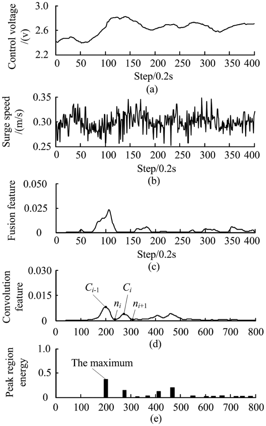
Experimental data and fault feature extraction results: (a) control voltage for thruster, (b) surge speed of AUV, (c) fusion feature extraction result, (d) convolution feature extraction result, and (e) peak region energy distribution.

Extract fusion feature

As shown in Figure 1, the fusion feature is extracted from surge speed and control voltage of AUV. The extraction steps, that is, sliding time window, wavelet decomposition, derivation operation, extract feature based on MB algorithm, and fuse feature based on evidence theory, are same to the ones of the FFMM method. The extracted fusion feature is shown in Figure 2(c).

Calculate convolution feature

Convolution feature from fusion feature by equation (4) is calculated.²³ The obtained convolution feature is shown in Figure 2(d)

T_{C} (n) = T_{F} (n) * T_{F} (n) = \sum_{j = 0}^{n} T_{F} (j) T_{F} (n - j)

(4)

where T_F(n) is fusion feature and T_C(n) is convolution feature.

Calculate PRE

As shown in Figure 2(d), to the peak C_i, n_i is the time step where the left adjacent trough locates, and n_i_+ 1 is the time step where the right adjacent trough locates. The PRE of peak C_i is calculated by equation (5)

E_{Ci} = \sum_{n = n_{i}}^{n_{i + 1}} T_{C} (n)

(5)

where E_Ci is the PRE of peak C_i and T_C(n) is convolution feature.

This procedure is repeated with every peak in the convolution feature. The PRE distribution is shown in Figure 2(e)

Extract fault feature

Extract fault feature from PRE distribution by equation (6)

F = max_{i} (E_{Ci})

(6)

where F is the fault feature extracted by the proposed PRE method and E_Ci is the PRE of peak C_i.

The effectiveness of the proposed method will be verified in section “Experimental validation of the PRE method.”

LSGRG method–based fault degree estimation

To further get an estimation result between adjacent standard fault degrees, a LSGRG method is proposed. The proposed method is developed from the GRA algorithm. The basic idea of the proposed method contains two steps, namely, first determine the fault degree interval and then calculate the fault degree within the interval. The flow chart of the proposed method is shown in Figure 3.

Figure 3.

Flow chart of the LSGRG method.

The detailed process of the LSGRG method is presented as follows.

Calculate the highest and second highest GRG between unknown mode vector and standard mode vectors

In Figure 3, the standard fault modes database and the calculation steps (i.e. sliding time window, create unknown mode vector based on PRE method, and calculate the GRG between unknown mode vector and standard mode vectors) are same to the ones of GRA algorithm.

Determine the two nearest standard mode vectors to unknown mode vector

Standard mode vector ${\bar{X}}_{M}$ and standard fault degree ${\bar{λ}}_{M}$ are corresponding to the highest GRG γ_M. Standard mode vector ${\bar{X}}_{S}$ and standard fault degree ${\bar{λ}}_{S}$ are corresponding to the second highest GRG γ_S. The standard mode vectors ${\bar{X}}_{M}$ and ${\bar{X}}_{S}$ are the two nearest standard mode vectors to unknown mode vector.

Calculate the GRG between standard mode vectors

According to step 2, the standard mode vectors ${\bar{X}}_{M}$ and ${\bar{X}}_{S}$ are the two nearest standard mode vectors to unknown mode vector. Correspondingly, unknown fault degree λ_U locates between standard fault degrees ${\bar{λ}}_{M}$ and ${\bar{λ}}_{S}$ . If λ_U locates at ${\bar{λ}}_{M}$ , the GRG between $X_{U}$ and ${\bar{X}}_{M}$ (given the symbol $γ'_{UM}$ ) is equal to the GRG between ${\bar{X}}_{M}$ and ${\bar{X}}_{M}$ (given the symbol $γ'_{MM}$ ). If λ_U locates at ${\bar{λ}}_{S}$ , the GRG $γ'_{UM}$ is equal to the GRG between ${\bar{X}}_{S}$ and ${\bar{X}}_{M}$ (given the symbol $γ'_{SM}$ ).

In this step, the GRG between standard mode vectors, that is, $γ'_{MM}$ and $γ'_{SM}$ , are calculated based on GRA algorithm.

Establish a mapping relationship between GRG and fault degree

According to the analysis in step 3, the mapping relationship between GRG $γ'_{UM}$ and unknown fault degree λ_U is established as equation (7)

λ_{U} = k \times γ'_{UM} + b

(7)

where k and b are parameters to be determined.

Next, the value of parameters k and b is determined. As known, when λ_U is equal to ${\bar{λ}}_{M}$ , $γ'_{UM}$ is equal to $γ'_{MM}$ . When λ_U is equal to ${\bar{λ}}_{S}$ , $γ'_{UM}$ is equal to $γ'_{SM}$ . Put $γ'_{MM}$ and ${\bar{λ}}_{M}$ a new equation, and then put $γ'_{SM}$ and ${\bar{λ}}_{S}$ into Equation (7) to get another new equation. The two new equations construct a system of equations. Solve the equations and obtain the value of parameters k and b.

Return the value of parameters k and b back to equation (7) and get the final form of the mapping relationship between GRG and fault degree expressed as equation(8)

λ_{U} = \frac{{\bar{λ}}_{M} - {\bar{λ}}_{S}}{{γ'}_{MM} - {γ'}_{SM}} γ'_{UM} + \frac{{\bar{λ}}_{S} \times {γ'}_{MM} - {\bar{λ}}_{M} \times {γ'}_{SM}}{{γ'}_{MM} - {γ'}_{SM}}

(8)

Calculate fault degree

Calculate the GRG between X _U and ${\bar{X}}_{M}$ , namely $γ'_{UM}$ . Put $γ'_{UM}$ into equation (8) and calculate the fault degree λ_U. The effectiveness of the proposed method will be verified in section “Experimental validation of the LSGRG method.”

Experimental validations

To verify the effectiveness of the proposed methods (i.e. the PRE method and the LSGRG method), pool experiments of the experimental prototype (i.e. Beaver II) are performed. In the following, Beaver II prototype and experimental condition, experimental validation of the PRE method, and experimental validation of the LSGRG method will be described in detail.

Beaver II prototype and experimental condition

Beaver II prototype

The Beaver II prototype is defined as an open-frame AUV, see Figure 4. The prototype configuration is composed of teflon plate and angle aluminum, 0.8 m long, 0.5 m wide, and 0.4 m high, equipped with two pressure vessels of the same dimensions, 0.6 m long and 0.2 m diameter. Its mass is 50 kg. The Beaver II is intrinsically stable in pitch and roll. The overall structure of the vehicle is symmetric with respect to the XZ planes. And the X-axis of the prototype is parallel to the axis of the vessels.

Figure 4.

Physical layout of the Beaver II AUV.

The Beaver II sensor system is composed of Doppler velocity log (DVL), digital compass, and depth meter, see Figure 4. The surge, sway, and heave speed are measured by the DVL whose update rate is 5 Hz. The heading, roll, and pitch position are measured by the digital compass whose update rate is 13 Hz. Depth measurement is achieved via the depth meter whose update rate is 20 Hz. The sensor data logging rate of the on-board computer system is 5 Hz.

The Beaver II propulsion system is composed of six brush thrusters, see Figures 4 and 5. The surge speed is controlled by thrusters HT3 and HT4 which are of the same specifications, DC24V rated voltage, and 200 W rated power. The heading is controlled by thrusters HT1 and HT2 which are of the same specifications, DC24V rated voltage, and 90 W rated power. The depth is controlled by thrusters VT1 and VT2 whose specifications are same as the ones of HT1 and HT2. All controllable degrees of freedom are controlled by a single closed-loop controller.

Figure 5.

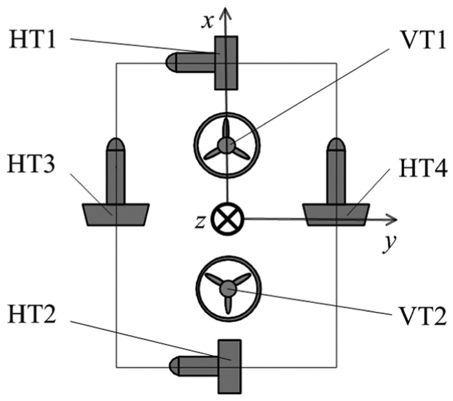
Thruster configuration of the Beaver II.

Experimental environment

Experiments are conducted in the pool which is 50 m long, 30 m wide, and 10 m depth. External disturbances (e.g. currents) are driven by the ocean current simulation device (see Figure 6). The ocean current simulation device is composed of angle aluminum and four brush thrusters which are of the same specifications, DC24V rated voltage, and 400 W rated power.

Figure 6.

Ocean current simulation device and process.

Thruster fault simulation method

In experiments, the thruster fault is simulated by software fault simulation method.²⁴ The basic theory and process of the method could be described as follows.

Establish the thruster model

The thruster model is used to reflect the relationship between output thrust and control voltage. To establish the thruster model, the whole thruster is put in the poll at bollard pull conditions, and the output thrust is measured corresponding to a set of control voltage. The results for HT3 are shown in Figure 7.

Figure 7.

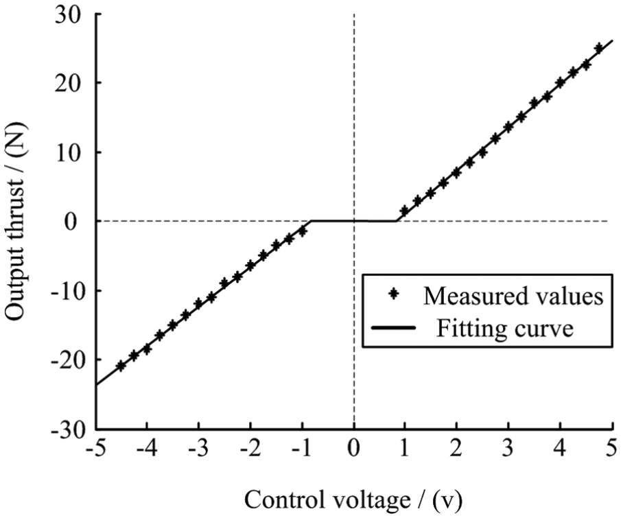
Relationship between output thrust and control voltage.

As shown in Figure 7, the relationship between output thrust and control voltage is nearly linear, so the thruster model for HT3 is established as equation (9). The coefficients in the thruster model are identified by least square method

τ = {\begin{matrix} 6.26 \times V - 5.26 & 0.84 < V \leq 5 \\ 0 & - 0.84 \leq V \leq 0.84 \\ 5.70 \times V + 4.81 & - 5 \leq V < - 0.84 \end{matrix}

(9)

where τ is the output thrust of thruster and V is the control voltage which is applied to the thruster driver.

Simulate the thruster fault

AUV thruster fault is generally characterized by losing output thrust.^3,24 Here, the fault degree describes the lost percent of output thrust.²⁵ For example, when the fault degree is λ, the ratio between the actual thrust τ′ and the desired thrust τ is 1 − λ, namely τ′ = (1 − λ) × τ. To simulate this, when AUV is moving forward, the control voltage which is actually applied to the thruster driver is calculated by equation (10)

V' = (1 - λ) \times V + 0.84 \times λ

(10)

where V′ is the control voltage which is applied to the thruster driver actually, V is the control voltage of the controller output, and λ is the fault degree.

Main parameters in the experiments

In all experiments, the surge speed controller outputs same control voltage for HT3 and HT4. The difference between the thruster models of HT3 and HT4 does cause the change of heading. But the change of heading will be compensated by the heading closed-loop controller. Experimental depth is 1 m.

In the experiments for the validation of the PRE method, AUV target surge speed is 0.3 m/s, from step 150 to the end, the HT3 carries with the simulated fault, and the fault degree is 30%. This procedure is repeated with the fault degree being 0%, 10%, 20%, and 40%. It is noted that fault degree being 0% means that thruster is fault free. In addition, the experiments are extended to AUV target surge speed being 0.2, 0.4, and 0.5 m/s.

In the experiments for the validation of the LSGRG method, AUV target surge speed is 0.3 m/s, from step 150 to the end, the HT3 carries with the simulated fault, and the fault degree is 15%. This procedure is repeated with the fault degree being 18%, 20%, 23%, 30%, and 34%. The standard fault modes database is established based on the experimental data in the validation of the PRE method. Therefore, the standard fault degrees are 0%, 10%, 20%, 30%, and 40%.

It must be emphasized that in the experiments for the validation of the PRE method and the LSGRG method, there exist the fault degrees at the same time, and they are all known to the authors as they are all simulated by software fault simulation method, but they have different meanings. The fault degrees in the experimental validation of the PRE method are known to the on-board computer system and are regarded as standard fault degrees. The fault degrees in the experimental validation of the LSGRG method are unknown to the on-board computer system and are to be estimated.

Experimental validation of the PRE method

The experimental data in the case of AUV surge target speed being 0.3 m/s and the fault degree being 0%, 10%, 20%, 30%, and 40%, respectively, are shown in Figure 8.

Figure 8.

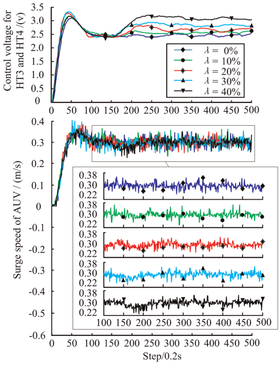
Experimental data in the case of AUV surge target speed being 0.3 m/s and the fault degree being 0%, 10%, 20%, 30%, and 40%.

As shown in Figure 8, from step 0 to step 100, AUV is in start-up. After step 101, AUV begins to move at a stable speed of 0.3 m/s. This article researches on thruster fault identification method for AUV at stable speed, so the data from step 101 to step 500 are selected to be analyzed. To verify the effectiveness of the proposed PRE method, both the proposed method and the FFMM method are used to extract fault feature from the experimental data.

The mapping relationship between fault feature and fault degree obtained by the FFMM method is shown in Figure 9(a) and the one obtained by the proposed method is shown in Figure 9(b). The computation cost of both methods is listed in Table 1.

Figure 9.

Mapping relationships obtained by different methods in the case of AUV surge speed being 0.3 m/s: (a) FFMM method and (b) proposed PRE method.

Table 1.

Computation cost of different fault feature extraction methods in AUV surge speed being 0.3 m/s case.

λ (%)	A _PRE (s)	A _FFMM (s)
0	0.01937	0.01889
10	0.01828	0.01783
20	0.01862	0.01818
30	0.01854	0.01812
40	0.01941	0.01898

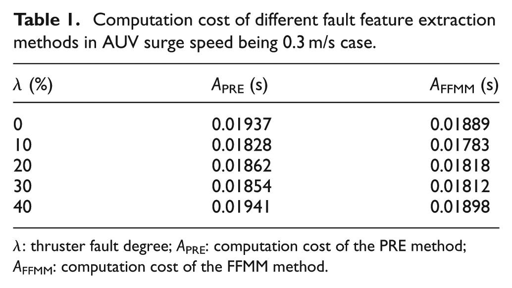
λ: thruster fault degree; A_PRE: computation cost of the PRE method; A_FFMM: computation cost of the FFMM method.

It must be emphasized that both the abscissas in Figure 9(a) and 9(b) are fault feature but they have different meanings. The abscissa in Figure 9(a) is the maximum of fusion feature. The abscissa in Figure 9(b) is the maximum of PRE.

As shown in Figure 9(a), the mapping relationship of fault feature and fault degree is non-monotonic and one fault feature is corresponding to multiple fault degrees. For example, according to the mapping relationship, when fault feature is equal to 0.025, the corresponding fault degrees are 7.3%, 16.1%, and 20.8%.

As shown in Figure 9(b), the mapping relationship of fault feature and fault degree is monotonic and one fault feature is corresponding to only one fault degree. For example, according to the mapping relationship, when fault feature is equal to 0.25, the corresponding fault degree is 12.7%.

As shown in Table 1, for fault degrees 0%, 10%, 20%, 30%, and 40%, the computation cost is 0.01937 s, 0.01828 s, 0.01862 s, 0.01854 s, and 0.01941 s for the PRE method, while it is 0.01889 s, 0.01783 s, 0.01818 s, 0.01812 s, and 0.01898 s for the FFMM method. The computation cost increases 2.5%, 2.5%, 2.4%, 2.3%, and 2.2% using the PRE method compared with the FFMM method.

In summary, the fault feature extracted by the proposed PRE method is monotonic to fault degree and one fault feature is corresponding to only one fault degree. While the fault feature extracted by the FFMM method is non-monotonic to fault degree and one fault feature is corresponding to multiple fault degrees. In addition, the computation cost of the PRE method is about 0.018 s and increases 2.2%–2.5% compared with the FFMM method.

Besides the case of AUV surge speed being 0.3 m/s, the cases of AUV surge speed being 0.2, 0.4, and 0.5 m/s are analyzed as well. The results are similar to each other, showing that the fault feature extracted by the PRE method is monotonic to fault degree while the one extracted by the FFMM method is not (see Figure 10). They also show that the computation cost of the PRE method is about 0.019 s and increases 2.1%–2.8% compared with the FFMM method (see Table 2).

Figure 10.

Mapping relationships obtained by different methods in the cases of AUV surge speed being 0.2, 0.4, and 0.5 m/s: (a) the FFMM method and (b) the proposed PRE method.

Table 2.

Computation cost of different fault feature extraction methods in AUV surge speed being 0.2, 0.4, and 0.5 m/s cases.

u (m/s)	λ (%)	A _PRE (s)	A _FFMM (s)
0.2	0	0.01885	0.01843
	10	0.01861	0.01821
	20	0.01928	0.01889
	30	0.01876	0.01835
	40	0.01908	0.01868
0.4	0	0.01886	0.01839
	10	0.01935	0.01890
	20	0.01830	0.01782
	30	0.01980	0.01937
	40	0.01862	0.01812
0.5	0	0.01945	0.01903
	10	0.01969	0.01927
	20	0.01872	0.01827
	30	0.01922	0.01879
	40	0.01911	0.01868

u: autonomous underwater vehicle surge speed; λ: thruster fault degree; A_PRE: computation cost of the peak region energy method; A_FFMM: computation cost of the fusion feature modulus maximum method.

Experimental validation of the LSGRG method

To verify the effectiveness of the proposed LSGRG method, both the proposed method and the GRA algorithm are applied to estimate fault degree. The experimental data in the case of AUV surge target speed being 0.3 m/s and the fault degree being 15%, 18%, 20%, 23%, 30%, and 34% are analyzed. The results are presented in Table 3.

Table 3.

Fault degree estimation results of different methods.

λ_U (%)	$\hat{λ}$ (%)	$λ'$ (%)	A _LSGRG (s)	A _GRA (s)
15	15.9	20	0.02149	0.02146
18	16.8	20	0.02204	0.02202
20	21.5	20	0.02152	0.02150
23	24.7	20	0.02218	0.02216
30	27.7	30	0.02094	0.02092
34	34.6	30	0.02194	0.02191

λ_U: unknown fault degree; $\hat{λ}$ : estimation results for the proposed least square grey relational grade method; $λ'$ : estimation results for the grey relational analysis algorithm; A_LSGRG: computation cost of the least square grey relational grade method; AGRA: computation cost of the grey relational analysis algorithm.

In case of unknown fault degree locating between adjacent standard fault degrees

As shown in Table 3, for the unknown fault degrees locating between adjacent standard fault degrees (i.e. 15%, 18%, 23%, and 34%), the fault degree estimation results are 15.9%, 16.8%, 24.7%, and 34.6% for the proposed method, while they are 20%, 20%, 20%, and 30% for the GRA algorithm. The experimental results indicate that the estimation results for the proposed method are additive fault degrees between adjacent standard fault degrees while the ones for the GRA algorithm are only ones of standard fault degrees. In addition, to compare the proposed method with the GRA algorithm in terms of identification accuracy, the identification accuracies of both methods are listed in Table 4.

Table 4.

Identification accuracies of different methods in case of unknown fault degree locating between adjacent standard fault degrees.

λ_U (%)	$\hat{p}$ (%)	$p'$ (%)
15	94.0	66.7
18	93.3	88.9
23	92.6	87.0
34	98.2	88.2

λ_U: unknown fault degree; $\hat{p}$ : identification accuracy of the proposed method; $p'$ : identification accuracy of the grey relational analysis algorithm.

As shown in Table 4, in terms of identification accuracy, for unknown fault degrees 15%, 17%, 25%, and 33%, the identification accuracies are 94.0%, 93.3%, 92.6%, and 98.2% for the proposed method, while they are 66.7%, 88.9%, 87.0%, and 88.2% for the GRA algorithm. The results show that the identification accuracies increase 40.9%, 4.9%, 6.4%, and 11.3% using the proposed method compared with the GRA algorithm.

In summary, the experimental results indicate that the proposed method can further get an additive fault degree between adjacent standard fault degrees and have higher identification accuracy in comparison to the GRA algorithm.

In case of unknown fault degree locating at standard fault degrees

In Table 3, the unknown fault degrees 20% and 30% locate at standard fault degrees. For the two unknown fault degrees, the identification accuracies of the proposed method and the GRA algorithm are shown in Table 5.

Table 5.

Identification accuracies of different methods in case of unknown fault degree locating at standard fault degrees.

λ_U (%)	$\hat{p}$ (%)	$p'$ (%)
20	92.5	100
30	92.3	100

λ_U: unknown fault degree; $\hat{p}$ : identification accuracy of the proposed method; $p'$ : identification accuracy of the grey relational analysis algorithm.

As shown in Tables 3 and 5, for unknown fault degrees 20% and 30%, the estimation results are 21.5% and 27.7% for the proposed method, while they are 20% and 30% for the GRA algorithm. Meanwhile, the identification accuracies are 92.5% and 92.3% for the proposed method, while they are 100% and 100% for the GRA algorithm. The experimental results indicate that the identification accuracies for the proposed method are beyond 92%, and they decrease 7.5% and 7.7% using the proposed method compared with the GRA algorithm.

In terms of the mean and standard deviation of identification accuracy

In practice, the fault degrees of thruster are stochastic, being the combination of the above two cases. As shown in Tables 4 and 5, for unknown fault degrees 15%, 18%, 20%, 23%, 30%, and 34%, the mean of identification accuracy is 93.8% for the proposed method while it is 88.5% for the GRA algorithm, showing the mean increases 6.0% using the proposed method compared with the GRA algorithm. Moreover, the standard deviation of identification accuracy is 2.2% for the proposed method while it is 12.2% for the GRA algorithm, showing the standard deviation decreases 82.0% using the proposed method compared with the GRA algorithm. The experimental results indicate that the proposed method is more effective in comparison to the GRA algorithm in terms of the both mean and standard deviation of identification accuracy.

In terms of computation cost of fault degree estimation method

As shown in Table 3, for fault degrees 15%, 18%, 20%, 23%, 30%, and 34%, the computation cost is 0.02149s, 0.02204s, 0.02152s, 0.02218s, 0.02094s, and 0.02194s for the proposed LSGRG method, while it is 0.02146s, 0.02202s, 0.02150s, 0.02216s, 0.02092s, and 0.02191s for the GRA algorithm. The computation cost increases 0.14%, 0.09%, 0.09%, 0.09%, 0.10%, and 0.14% using the LSGRG method compared with the GRA algorithm.

Conclusion

The problem of AUV thruster fault identification is researched in this article. Since the fault feature extracted by the FFMM method is non-monotonic to fault degree, the PRE method is proposed. Considering the fault degree estimation result of the GRA algorithm is just one of standard fault degrees, the LSGRG method is proposed. The results in the pool experiments show that the PRE method can extract the fault feature whose value is monotonic to fault degree at the expense of 2.1%–2.8% more computation cost than the FFMM method. The LSGRG method can further obtain an additive fault degree between adjacent standard fault degrees. It increases the mean of identification accuracy by 6.0% and decreases the standard deviation of identification accuracy by 82.0% at the expense of 0.09%–0.14% more computation cost than the GRA algorithm.

Footnotes

Academic Editor: Jia-Jang Wu

Declaration of conflicting interests

The author(s) declared no potential conflicts of interest with respect to the research, authorship, and/or publication of this article.

Funding

The author(s) disclosed receipt of the following financial support for the research, authorship, and/or publication of this article: The work is supported by the National Natural Science Foundation of China (No. 51279040) and Basic Research Program of Ministry of Industry and Information Technology of People’s Republic of China (No. B2420133003).

References

Dearden

Ernits

Automated fault diagnosis for an autonomous underwater vehicle. IEEE J Oceanic Eng 2013; 38: 484–499.

Ismail

Faudzi

Dunnigan

AW.

Fault-tolerant region-based control of an underwater vehicle with kinematically redundant thrusters. Math Probl Eng 2014; 2014: 1–2.

Omerdic

Roberts

Thruster fault diagnosis and accommodation for open-frame underwater vehicles. Control Eng Pract 2004; 12: 1575–1598.

Liu

Zhu

Yang

SX.

Unmanned underwater vehicles fault identification and fault-tolerant control method based on FCA-CMAC neural networks, applied on an actuated vehicle. J Intell Robot Syst 2012; 66: 463–475.

Zhang

Wang

. Thruster fault diagnosis in autonomous underwater vehicle based on grey qualitative simulation. Ocean Eng 2015; 105: 247–255.

Wang

Tang

. An improved method based on CEEMD for fault diagnosis of rolling bearing. Adv Mech Eng. Epub ahead of print 18 November 2014. DOI: 10.1155/2014/676205.

Zhang

Yin

Liu

. Feature extraction and fusion for thruster faults of AUV with random disturbance. J Huazhong Univ Sci Technol Nat Sci Ed 2015; 43: 22–26.

Wang

Wan

. Sensor fault diagnosis for underwater robots. In: Proceedings of the 7th world congress on intelligent control and automation, Chongqing, China, 25–27 June 2008, pp.254–259. New York: IEEE.

Zhang

Wang

YJ.

A method of multi-sensor simultaneous fault detection for autonomous underwater vehicle. Robotica 2010; 32: 298–305.

10.

Miskovic

Barisic

. Fault detection and localization on underwater vehicle propulsion systems using Principal Component Analysis. In: Proceedings of the IEEE international symposium on industrial electronics 2005, Dubrovnik, 20–23 June 2005, pp.1721–1727. New York: IEEE.

11.

Jia

Wang

. Fault diagnosis based on second-order Taylor series dynamic prediction for autonomous underwater vehicle sensor. In: Proceedings of 2013 Chinese automation congress, Changsha, China, 7–8 November 2013, pp.651–655. New York: IEEE.

12.

Feng

Zuo

Hao

. Gear damage assessment based on cyclic spectral analysis. IEEE T Reliab 2011; 60: 21–32.

13.

Shen

Chen

. A monotonic degradation assessment index of rolling bearings using fuzzy support vector data description and running time. Sensors 2012; 12: 10109–10135.

14.

Lei

Zuo

. A multidimensional hybrid intelligent method for gear fault diagnosis. Expert Syst Appl 2010; 37: 1419–1430.

15.

Yan

Jiang

. A new data mining approach for gear crack level identification based on manifold learning. Mechanics 2012; 18: 29–34.

16.

Cheng

Zhang

XF.

Crack level estimation approach for planetary gearbox based on simulation signal and GRA. J Sound Vib 2012; 331: 5853–5863.

17.

Wulandhari

Wibowo

Desa

MI.

Improvement of adaptive GAs and back propagation ANNs performance in condition diagnosis of multiple bearing system using grey relational analysis. Comput Intell Neurosci 2014; 2014: 419743.

18.

Zhang

Chu

ZZ.

Multi-fault diagnosis for autonomous underwater vehicle based on fuzzy weighted support vector domain description. China Ocean Eng 2014; 28: 1–18.

19.

Zhang

. Gear fault diagnosis method using ensemble empirical mode decomposition energy distribution and grey similar incidence. J Mech Eng 2014; 50: 70–77.

20.

Zeng

Qiu

Liu

. Research on equipment degradation state recognition and fault prognostics method based on KPCA-hidden semi-Markov model. Chin J Sci Instrum 2009; 30: 1341–1346.

21.

Lei

Zuo

MJ.

Gear crack level identification based on weighted K nearest neighbor classification algorithm. Mech Syst Signal Pr 2009; 23: 1535–1547.

22.

Moosavian

Khazaee

Najafi

. Spark plug fault recognition based on sensor fusion and classifier combination using Dempster–Shafer evidence theory. Appl Acoust 2015; 93: 120–129.

23.

Zhao

Lin

Wang

. Fluctuation analysis of instantaneous angular speed based on digital differentiator and its application in vibration source identification. J Mech Eng 2012; 48: 1–6.

24.

Chu

Zhang

MJ.

Fault reconstruction of thruster for autonomous underwater vehicle based on terminal sliding mode observer. Ocean Eng 2014; 88: 426–434.

25.

Zhao

Skjetne

Blanke

. Particle filter for fault diagnosis and robust navigation of underwater robot. IEEE T Contr Syst T 2014; 22: 2399–2407.

Thruster fault identification method for autonomous underwater vehicle using peak region energy and least square grey relational grade

Abstract

Keywords

Introduction

Problem statement

Fault feature value is non-monotonic to thruster fault degree

Fault degree estimation result is only one of standard fault degrees

PRE method–based fault feature extraction

Extract fusion feature

Calculate convolution feature

Calculate PRE

Extract fault feature

LSGRG method–based fault degree estimation

Calculate the highest and second highest GRG between unknown mode vector and standard mode vectors

Determine the two nearest standard mode vectors to unknown mode vector

Calculate the GRG between standard mode vectors

Establish a mapping relationship between GRG and fault degree

Calculate fault degree

Experimental validations

Beaver II prototype and experimental condition

Beaver II prototype

Experimental environment

Thruster fault simulation method

Establish the thruster model

Simulate the thruster fault

Main parameters in the experiments

Experimental validation of the PRE method

Experimental validation of the LSGRG method

In case of unknown fault degree locating between adjacent standard fault degrees

In case of unknown fault degree locating at standard fault degrees

In terms of the mean and standard deviation of identification accuracy

In terms of computation cost of fault degree estimation method

Conclusion

Footnotes

Declaration of conflicting interests

Funding

References