Sage Journals: Discover world-class research

Abstract

The thermal problem of plate slides against symmetrically located contacting pads is investigated. The aim is to find out the influences of plate thickness, moving speed, and convection on the temperature field of the plate. Proper models and computing methods for specific situations can be determined based on these analyses. Finite element method of moving heat input is used to calculate the temperature field which is validated by comparing with some existing analytical solutions. The results show that the characteristic time for the steady state of temperature can be approximated exponentially as a function of moving speed. If the plate is thinner than the critical thickness, the surface temperature is increased significantly, which means that the temperature field is very sensitive to the plate thickness in this situation. The increasing moving speed increases the peak surface temperature almost linearly, and the convection outside of the contact area can decrease the peak surface temperature significantly if the heat sources move slowly, while it hardly affects the peak surface temperature if the heat sources move fast. Based on these results, the criterion of choosing a model and computing methods for studying the temperature fields in the similar structures is established.

Keywords

Conduction moving heat source finite element analysis mechanical modeling finite thickness plate

Introduction

For practical disk brakes and some plate grinding structures, they can be simplified to be a model of finite thickness plate that slides against two symmetrically located contacting pads as shown in Figure 1(a). The plate is heated in the contact area and cooled outside by convection. Symmetrically distributed temperature field in the plate can be produced in this process. In the sliding direction, the non-uniform temperature distribution between inside and outside of the contact area may induce surface deflections and results in hot spots^1–3 and thermal buckling.^4,5 Many researches on transient temperature fields of this model were conducted theoretically and experimentally.^6,7 Generally, when the plate is thick enough, the contact area can be treated as a semi-infinite model for the temperature analysis. The pioneer work was presented by Jaeger⁸ who derived analytical solutions of the temperature field in a semi-infinite body caused by a heat strip. Tseng et al.⁹ provided the thermal stress solutions for the semi-infinite model, and they are applied in some researches of disk brakes.^10–12 Aderghal et al.¹³ studied the influences of moving speed of the heat source and the cooling effects on the temperature field numerically. Some researches considered the plate thickness in given structures and studied the temperature of the plate by simulation or experiments.^14–18 But, these researches treated the heat source as independent of the moving speed. In the sliding process, the heat strength is actually a function of the moving speed with a constant pressure, so the influences of moving speed should be considered. It is reasonable to treat the plates as finite thickness model in any structure and apply numerical methods to calculate the temperature field, but it is inefficient to do so. The analytical solution for semi-infinite model can get the solutions quickly, while the structure and working conditions should be checked before modeling in order to make the calculation accurate.

Figure 1.

(a) The model of plate slides against two symmetrically located pads. (b) Simplified heat transfer model of the plate with finite thickness. (c) Simplified heat transfer model of the plate with semi-infinite thickness.

This work aims to study the influences of plate thickness, moving speed, and convection outside of the contact area on the temperature field, based on which the criterion of modeling can be set up. Finite element method (FEM) is used to study the temperature field in this work. A new dimensionless temperature is introduced, and the heat source strength depending on the moving speed is considered. The characteristic time of steady state is investigated first and followed by the other three factors.

Model

Statement of the problem

The two-dimensional (2D) model is presented in Figure 1(a), where the pads are symmetrically located on the plate surfaces. The actuating pressure P is applied uniformly on the pads and the plate slides with speed V. In this situation, the mid-plane of the disk can be considered as adiabatic due to the symmetrically heating, and a simplified general thermal model of the disk can be set up as shown in Figure 1(b). The contact area is represented by a moving heat source with 2l in length, and a moving Cartesian coordinate system xoy is fixed at the center. The cooling effect outside of the contact area is represented by the convective heat transfer coefficient h. The considered model length 2L is much longer than the heat source width 2l, so that the vertical boundaries Γ₁ and Γ₃ are set to be adiabatic. If the plate is thick enough, it can be considered as semi-infinite as shown in Figure 1(c).

Solution of the finite thickness model

The plate material is isotropic and uniform. There is no inner heat source in the plate, and the radiation is ignored. The transient heat conduction equation in the moving coordinate system is¹⁹

κ (\frac{\partial^{2} T}{\partial x^{2}} + \frac{\partial^{2} T}{\partial y^{2}}) = \frac{\partial T}{\partial t} + V \frac{\partial T}{\partial x}

(1)

where κ = λ/(ρc) is the thermal diffusivity of the material. In the finite thickness model, Newton’s law of cooling is applied and the boundary conditions are

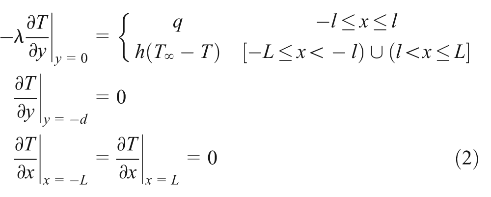
\begin{matrix} - λ {\frac{\partial T}{\partial y} |}_{y = 0} = {\begin{matrix} q - l \leq x \leq l \\ h (T_{\infty} - T) [- L \leq x < - l) \cup (l < x \leq L] \end{matrix} \\ {\frac{\partial T}{\partial y} |}_{y = - d} = 0 \\ {\frac{\partial T}{\partial x} |}_{x = - L} = {\frac{\partial T}{\partial x} |}_{x = L} = 0 \end{matrix}

(2)

where T_∞ is the adiabatic wall temperature which equals to the initial temperature T ₀. q = DµPV is the heat flux that flows into the plate. D is the heat partition coefficient which has relationship with the contacting materials and varies in the interval of (0, 1).¹⁷ For the sake of generality, we introduce some dimensionless parameters: $x^{*} = x / L_{re}$ , $y^{*} = y / L_{re}$ , $l^{*} = l / L_{re}$ , $t^{*} = κ t / L_{re}^{2}$ , $Pe = V L_{re} / κ$ , $Bi = h L_{re} / λ$ , $T_{r} = q L_{re} / λ$ , and $T^{*} = (T - T_{0}) / T_{r}$ , where L_re is the characteristic length which can be any nonzero value. Pe and Bi are Peclet number and Biot number which represent the moving speed of the heat source and the convection on the boundaries, respectively. The dimensionless form of equation (1) can be written as

\frac{\partial^{2} T^{*}}{\partial {x^{*}}^{2}} + \frac{\partial^{2} T^{*}}{\partial {y^{*}}^{2}} = \frac{\partial T^{*}}{\partial t^{*}} + Pe \frac{\partial T^{*}}{\partial x^{*}}

(3)

Choosing the width of the heat source to be the characteristic length, that is, L_re = 2l, the dimensionless boundary conditions correspond to equations (2) are

\begin{matrix} - {\frac{\partial T^{*}}{\partial y^{*}} |}_{y^{*} = 0} = {\begin{matrix} 1 - 1 \leq x^{*} \leq 1 \\ - Bi T^{*}, (- \frac{L}{2 l} \leq x^{*} < - 1) \cup (1 < x^{*} \leq \frac{L}{2 l}) \end{matrix} \\ {\frac{\partial T^{*}}{\partial y^{*}} |}_{y^{*} = - \frac{d}{2 l}} = 0 \\ {\frac{\partial T^{*}}{\partial x^{*}} |}_{x^{*} = - \frac{L}{2 l}} = {\frac{\partial T^{*}}{\partial x^{*}} |}_{x^{*} = \frac{L}{2 l}} = 0 \end{matrix}

(4)

This problem can be solved by FEM. With the boundary conditions (4), the equivalent integral of this problem can be written as

\begin{matrix} \int_{Ω} u (\frac{\partial^{2} T^{*}}{\partial {x^{*}}^{2}} + \frac{\partial^{2} T^{*}}{\partial {y^{*}}^{2}} - \frac{\partial T^{*}}{\partial t^{*}} - Pe \frac{\partial T^{*}}{\partial x^{*}}) d Ω \\ + \int_{Γ_{2}} \bar{u} (λ \frac{\partial T^{*}}{\partial x} n_{x} + λ \frac{\partial T^{*}}{\partial y} n_{y} + 1 + Bi T^{*}) d Γ_{2} = 0 \end{matrix}

(5)

where n_x and n_y are the normal vectors of the boundaries, and Ω is the area of the cross-section. In each element, the temperature T ^* is approximated as

T^{*} \approx \sum_{i = 1}^{n} N_{i} (x^{*}, y^{*}) T_{i}^{*} (t)

(6)

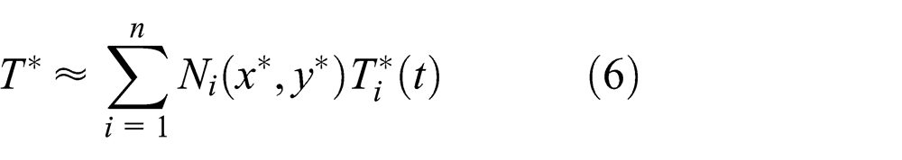
where N_i (x^* , y^* ) are the shape functions and $T_{i}^{*} (t)$ are the nodal temperatures. With Galerkin’s method, the weight functions u and $\bar{u}$ are chosen to be the shape functions on the boundaries which is $\bar{u} = - u = N_{j}$ . The matrix form of this problem can be written as

([K_{k}] + [K_{c}]) {T^{*}} = - [C] {{\overset{\cdot}{T}}^{*}} + {R_{q}} + [K_{c}] {T_{\infty}^{*}}

(7)

where $[K_{k}]$ , $[K_{c}]$ , $[C]$ , and ${R_{q}}$ are the conductivity matrix, convection matrix, capacity matrix, and heat flux input vector, respectively. Equation (7) is solved by direct integration, and the unconditional stable backward differential method is applied

{{\overset{\cdot}{T}}^{*} (t + Δ t)} = {{\overset{\cdot}{T}}^{*}}_{t (n + 1)} = \frac{〈 {T^{*}}_{t (n + 1)} - {T^{*}}_{t (n)} 〉}{Δ t}

(8)

Substituting equation (8) into (7), the iteration form is then obtained

\begin{matrix} 〈 [C] + Δ t ([K_{k}] + [K_{c}]) 〉 {T^{*}}_{t (n + 1)} = [C] {T^{*}}_{t (n)} \\ + 〈 {R_{q}} + [K_{c}] {T_{e}^{*}} 〉 Δ t \end{matrix}

(9)

A FEM solver for the temperature field is developed based on equation (9) combined with the boundary and initial conditions.

Analytical solution of the semi-infinite model

The analytical solution of the semi-infinite model is provided by the literature⁸

\begin{matrix} T^{*} (x^{*}, y^{*}, t^{*}) = \frac{1}{2 \sqrt{π}} \\ \int_{0}^{t^{*}} e^{- \frac{{y^{*}}^{2}}{4 Fo}} [\erf (P_{+}) - \erf (P_{-})] \frac{1}{\sqrt{Fo}} dFo \end{matrix}

(10)

where erf(x) is the error function, $P_{+} = (x^{*} + l - PeFo) / (2 \sqrt{Fo})$ and $P_{-} = (x^{*} - l - PeFo) / (2 \sqrt{Fo})$ . The dimensionless Fourier number $Fo = κ (t - t') / L_{re}^{2}$ equals zero when t′ = t and equals t ^* when t′ = 0. By setting y ^* = 0, the surface temperature can be obtained

T^{*} (x^{*}, 0, t^{*}) = \frac{1}{2 \sqrt{π}} \int_{0}^{t^{*}} [\erf (P_{+}) - \erf (P_{-})] \frac{dFo}{\sqrt{Fo}}

(11)

In static situation, the heat source is kept stationary and the surface temperature can be figured out with equation (11) by setting Pe = 0 which gives

\begin{matrix} T^{*} (x^{*}, 0, t^{*}) = \frac{1}{2 \sqrt{π}} \\ \int_{0}^{t^{*}} [\erf (X_{+}) - \erf (X_{-})] \frac{dFo}{\sqrt{Fo}} \\ = \sqrt{\frac{t^{*}}{π}} [\begin{matrix} \erf (A_{1 +}) + \erf (A_{1 -}) \\ - A_{2 +} Ei (A_{3 +}) - A_{2 -} Ei (A_{3 -}) \end{matrix}] \end{matrix}

(12)

where $X_{+} = (x^{*} + l) / (2 \sqrt{Fo})$ , $X_{-} = (x^{*} - l) / (2 \sqrt{Fo})$ , $A_{1 +} = (l + x^{*}) / (2 \sqrt{t^{*}})$ , $A_{1 -} = (l - x^{*}) / (2 \sqrt{t^{*}})$ , $A_{2 +} = (l + x^{*}) / (2 \sqrt{π t^{*}})$ , $A_{2 -} = (l - x^{*}) / (2 \sqrt{π t^{*}})$ , $A_{3 +} = - {(l + x^{*})}^{2} / 4 t^{*}$ , and $A_{3 -} = - {(l - x^{*})}^{2} / 4 t^{*}$ .

When convection takes place on the surface of the semi-infinite model, the analytical solution provided by the literature¹³ takes the form

\begin{matrix} T^{*} (x^{*}) = - Bi \int_{- \infty}^{- l} T^{*} (s) K (x^{*}, s) ds \\ + \int_{- l}^{l} K (x^{*}, s) ds - Bi \int_{l}^{\infty} T^{*} (s) K (x^{*}, s) ds \end{matrix}

(13)

where $K (x^{*}, s) = 1 / π \exp (Pe / 2 (x^{*} - s)) K_{0} (Pe / 2 | x^{*} - s |)$ , and K ₀ is the modified Bessel function of the second kind of order zero.

Comparison of the solutions in semi-infinite model

If the plate thickness is large enough, the surface temperature of the finite thickness model should coincide with the analytical solution. In the FEM solver, four-node quadrilateral element is used. The plate is made from 65Mn steel whose physical properties λ, ρ, and c just vary a little when the temperature increases from 20°C to 300°C. For simplification, these material properties are considered to be constant and the values in room temperature (20°C) are used as listed in Table 1.

Table 1.

Properties of the plate material.

Thermal conductivity, λ (W/(m K))	42
Density, ρ (kg/m³)	7800
Specific heat, c (J/(kg K))	452

In the FEM solver, four-node quadrilateral element is used. The surface temperature profiles at four instants in static and moving situations are calculated with the analytical and numerical methods, and they are displayed in Figure 2(a) and (b), respectively. Figure 2(c) shows the comparison of these two methods when convection is applied on the surface when the steady state is just achieved (Pe = 1, Bi = 1).

Figure 2.

Comparison of the surface temperature calculated by finite element method (FEM) solver and the analytical solutions: (a) static heat source situation, (b) moving heat source situation, and (c) convection situation.

Some of the corresponding values of these subfigures are listed in Tables 2 –4, respectively, where $T_{A}^{*}$ is the analytical value and $T_{B}^{*}$ is the numerical value. It shows that the numerical results agree very well with the analytical solutions, hence the FEM solver is validated for calculating the temperatures with moving heat source and convection on the surface.

Table 2.

Comparison of the analytical and numerical values for the static situation as shown in Figure 2(a).

Time	x ^*	−4	−3	−2	−1	0	1	2	3	4
t ^* = 1	$T_{A}^{}$*	0.00251	0.01868	0.10181	0.54528	0.91973	0.54528	0.10181	0.01868	0.00251
	$T_{N}^{}$*	0.00275	0.01809	0.09637	0.53055	0.89965	0.53055	0.09637	0.01809	0.00275
t ^* = 2	$T_{A}^{}$*	0.02029	0.06982	0.21265	0.72289	1.12783	0.72289	0.21265	0.06982	0.02029
	$T_{N}^{}$*	0.01921	0.06611	0.20426	0.70949	1.11221	0.70949	0.20426	0.06611	0.01921
t ^* = 3	$T_{A}^{}$*	0.04755	0.12271	0.29777	0.83627	1.25264	0.83627	0.29777	0.12271	0.04755
	$T_{N}^{}$*	0.04698	0.12086	0.29412	0.83093	1.24662	0.83093	0.29412	0.12086	0.04698
t ^* = 4	$T_{A}^{}$*	0.07731	0.17082	0.36564	0.91973	1.34213	0.91973	0.36564	0.17082	0.07731
	$T_{N}^{}$*	0.07552	0.16747	0.36051	0.91317	1.33492	0.91317	0.36051	0.16747	0.07552

Table 3.

Comparison of the analytical and numerical values for the moving situation as shown in Figure 2(b).

Time	x ^*	−4	−3	−2	−1	0	1	2	3	4
t ^* = 1	$T_{A}^{}$*	0.03645	0.11728	0.28831	0.69243	0.74922	0.27016	0.01364	0.00081	0.00004
	$T_{N}^{}$*	0.03257	0.11268	0.28649	0.68869	0.75258	0.27194	0.01492	0.00241	0.00025
t ^* = 2	$T_{A}^{}$*	0.19792	0.31410	0.46898	0.81422	0.80832	0.29055	0.01862	0.00167	0.00015
	$T_{N}^{}$*	0.19309	0.30957	0.46212	0.80673	0.82187	0.32034	0.02367	0.00212	0.00058
t ^* = 3	$T_{A}^{}$*	0.31077	0.40162	0.52501	0.84373	0.82103	0.29503	0.01991	0.00198	0.00021
	$T_{N}^{}$*	0.30599	0.39518	0.51285	0.83396	0.82854	0.31661	0.02069	0.00209	0.00072
t ^* = 4	$T_{A}^{}$*	0.36022	0.43267	0.54196	0.85173	0.82433	0.29620	0.02027	0.00208	0.00023
	$T_{N}^{}$*	0.35588	0.42751	0.53377	0.84421	0.82596	0.30831	0.02067	0.00287	0.00077

Table 4.

Comparison of the analytical and numerical values for the situation in Figure 2(c) (Pe = 1, Bi = 1).

x ^*	−4	−3	−2	−1	0	1	2	3	4
$T_{A}^{}$*	0.105	0.159	0.272	0.860	1.041	0.405	0.048	0.015	0.006
$T_{N}^{}$*	0.103	0.157	0.269	0.845	1.038	0.397	0.047	0.014	0.003

Analysis of temperature field in the plate

Steady state

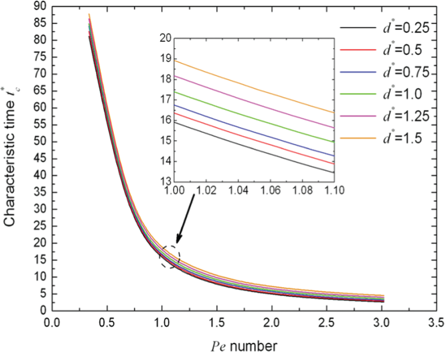
When the heat source moves with a constant speed, the surface temperature around the contact area is going to reach a steady state in the moving coordinate system.¹³ Defining temperature variation ratio $Δ T_{c}^{*} = (T_{t + Δ T}^{*} - T_{t}^{*}) / T_{t + Δ T}^{*} \times 100 %$ , the steady state is supposed to be achieved when $Δ T_{c}^{*} \leq 0.1 %$ , and the corresponding time is called the characteristic time $t_{c}^{*}$ . When there is no convection on the surface outside of the contact area, the variation of $t_{c}^{*}$ as function of Peclet number for several disk thicknesses are depicted in Figure 3. It shows that the variation processes of $t_{c}^{*}$ for all of these thickness values are similar and close to each other as d^* increases in the interval of [0.25, 1.5]. $t_{c}^{*}$ drops sharply from infinity to as low as 10 when Pe increases from 0 to 1.5, but decreases slowly when Pe > 1.5.

Figure 3.

Characteristic time of the steady state.

The variation curves in Figure 3 can be fitted as

t_{c}^{*} = AP e^{- B}

(14)

and the values of A and B for different thicknesses are listed in Table 5. It tells that the fitting curves agree excellent with the original data. Based on this relationship, when the heat source is moving slowly, it takes a long time to arrive at steady state and the characteristic time is very sensitive to the moving speed. When the heat source is moving fast, the temperature field will arrive at steady state quickly and they are not influenced too much by the plate thickness and the Peclet number.

Table 5.

Fitting parameter values in equation (13).

d ^*	0.25	0.5	0.75	1	1.25	1.5
A	14.63	15.21	15.91	16.68	17.59	18.61
B	1.56	1.52	1.49	1.44	1.39	1.34
R ²	0.999	0.999	0.999	0.998	0.997	0.996

Temperature field with new dimensionless system

Taking d^* = 0.5, for example, the dimensionless temperatures T^* with several Peclet numbers are evaluated and shown in Figure 4(a) when the steady state is just arrived. It shows that in the contact area −1 ≤ x^* ≤ 1, the surface temperature is higher than that of the mid-plane, and both of them become to be the same gradually after the contact area. Here exists a flat stage F after the contact area, which means that the temperature in this area has become uniform in the thickness. These flat stages are caused by the adiabatic boundaries of the surface and mid-plane. The dimensionless temperatures become lower and lower as the Peclet number increases in the current dimensionless system. Since the heat intensity depends on the moving speed, according to the definitions T^* = (T – T ₀)/T_r, T_r = qL_re /λ and Pe = VL_re /κ, the real temperature field in the plate can be expressed as

T = \frac{D μ p}{ρ c} Pe T^{*} + T_{0}

(15)

Figure 4.

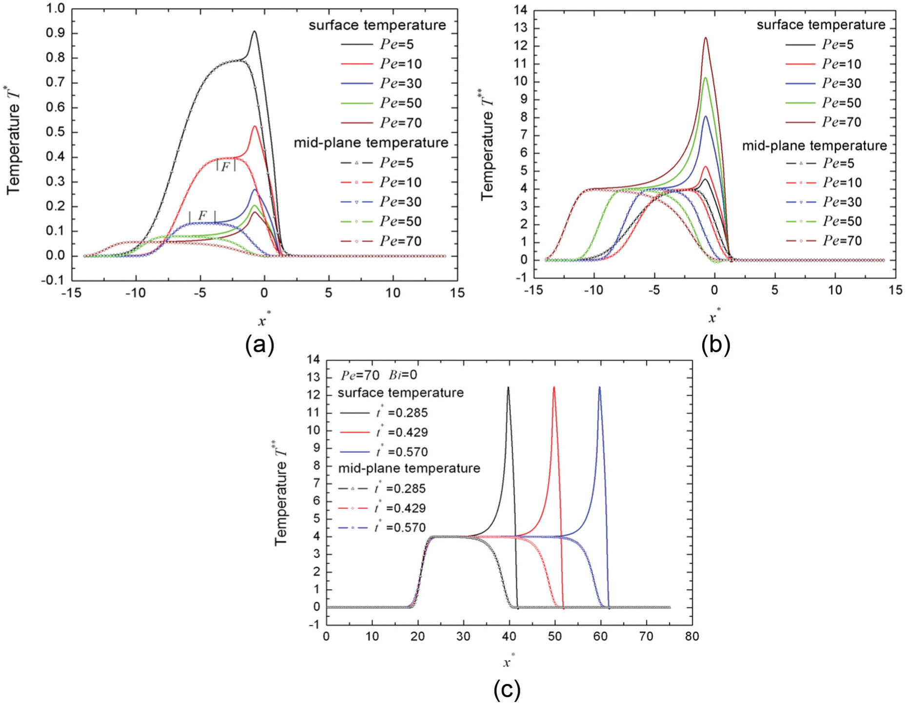
Moving speed influences on the surface and mid-plane temperatures when d^* = 0.5: (a) in the dimensionless system of T^* , (b) in the new dimensionless system of T^** , and (c) surface and mid-plane temperatures at three steady state instants when Pe = 70 and Bi = 0.

Introduce a new dimensionless temperature T^** = PeT^* , which includes the moving speed of the heat source and reflects the real temperature directly. The curves in Figure 4(a) then can be re-plotted in Figure 4(b) with T^** . Different from the dimensionless temperature T^* , the peak surface temperature $T_{smax}^{* *}$ in Figure 4(b) gets higher and higher when Pe increases, but all of the “flat stages”F for each Pe value have the same value of $T_{mmax}^{* *} = 3.95$ , which is the maximum temperature of the mid-plane. The surface and mid-plane temperatures at three steady state instants are shown in Figure 4(c) when Pe = 70 and Bi = 0. It shows that both of the temperatures no longer change after the steady state has been arrived, and only the “flat stage” is extended along the sliding direction. It can be concluded that for given plate thickness, the peak surface temperature increases with the moving speed, but the surface and mid-plane have the same temperature level after the contact area, no matter how fast the heat source is moving.

Influence of plate thickness and moving speed on the temperatures

The surface and mid-plane temperatures in the interval of −7 ≤ x^* ≤ 7 are depicted in Figure 5 after the steady state has been achieved. When d^* = 0.25, the surface and mid-plane temperatures have very tiny differences in the contact area as shown in Figure 5(a), which means the temperature field in the disk can be considered as uniformly distributed in the thickness. The temperatures after the contact area are raised up significantly compared with that before the contact area. When the disk becomes thicker to d^* = 0.5, the temperature differences between the surface and mid-plane are enlarged, and the temperatures after the contact area are decreased a half compared with that when d^* = 0.25. For even thicker plates as shown in Figure 5(b), the temperature differences are further enlarged. When d^* increases a lot from 3 to 12.5, $T_{smax}^{* *}$ only drops a little from 1.35 to 1.28 which means the thickness does not affect the surface temperature too much. The mid-plane temperature decreases to zero when d^* = 12.5, which means the disk is so thick that it can be treated as semi-infinite around the contact area. The surface temperature in this situation can be evaluated by the analytical solutions, which is much efficient than the FEM calculations.

Figure 5.

Surface and mid-plane temperatures in the disk with different thicknesses when Pe = 1 and Bi = 0: (a) thinner disks and (b) thicker disks.

In the contact area of [−1, 1], the surface temperature is raised up greatly in a short distance, so the peak surface temperature $T_{smax}^{* *}$ is important to characterize the thermal status of the plate. According to the temperature profiles in Figure 5, the variation of $T_{smax}^{* *}$ as function of thicknesses and Peclet numbers are displayed in Figure 6(a) and (b), respectively. For a given Peclet number, when the thickness d^* is thinner than a critical value, $T_{smax}^{* *}$ increases rapidly which tells that the peak surface temperature is very sensitive to the thickness. When d^* is thicker than the critical value, $T_{smax}^{* *}$ is kept at a constant value which means the plate thickness has little influence on the peak surface temperature. The critical thicknesses for each Peclet number are on the curve C, which tells that when the moving speed gets higher, the critical thickness becomes smaller. The left part of the curve C is called the sensitive area and the right part is called the non-sensitive area. In the sensitive area, the disk should be treated as finite thickness model because a tiny change in the thickness may induce large differences of the peak surface temperature. Also, the temperature field should be calculated with numerical methods. In the non-sensitive area, the disk can be treated as semi-infinite model, and the surface temperature can be evaluated by the analytical solutions no matter the heat source is moving fast or slow.

Figure 6.

Variation of the peak surface temperature $T_{smax}^{* *}$ for different thicknesses and Pe numbers: (a) the variation of $T_{smax}^{* *}$ as function of thickness and (b) the variation of $T_{smax}^{* *}$ as function of Pe number.

The corresponding increase in $T_{smax}^{* *}$ with respect to the Peclet number is presented in Figure 6(b). When the plate thickness d^* = 0.25, the peak surface temperature increases linearly, while it drops a lot when d^* = 0.5. When the thicknesses d^* equals two and six, the temperatures are very close to each other at any moving speed. When the heat source moves slowly, the peak surface temperature is influenced by the thickness of the disk. When the heat source moves fast especially for Pe > 10, all the peak surface temperatures are increasing linearly with the moving speed.

Influence of convection on the temperature field

The temperature contours in the plate are shown in Figure 7 where Pe = 30 and Bi = 0, 1, 10, and 20, respectively. In these plots, x′^* = x′/L_re and y′^* = y′/L_re are the dimensionless fixed coordinates, respectively. It shows that the temperature becomes uniform in the thickness after the contact area and the “flat stage” is obvious (12 < x ^′* < 16) in the adiabatic situation (Bi = 0). When convection is applied outside of the contact area (Bi = 1), the surface temperature after the contact area drops to be even lower than that of the mid-plane. When Bi = 20, the temperature field just varies a little from that with Bi = 10, which means the cooling effects can hardly make differences on the temperature field when it is strong enough.

Figure 7.

Temperature fields in the plate when Pe = 30, Bi = 0, 1, 10, and 20.

The corresponding surface and mid-plane temperature profiles are presented in Figure 8(a). When Pe = 30, although the cooling effect can make the surface temperature after the contact area to be lower than the mid-plane temperature, it scarcely influences the temperatures in the contact area [−1 < x^* < 1], no matter how strong the convection is. For higher moving speed Pe = 50 and Pe = 70, similar temperature profiles are obtained as shown in Figure 8(b) and (c) with higher peak surface temperatures. All the temperatures in the contact area can be represented by that in the adiabatic situation (Bi = 0).

Figure 8.

Surface and mid-plane temperatures under different cooling conditions with three Peclet numbers: (a) Pe = 30, (b) Pe = 50, and (c) Pe = 70.

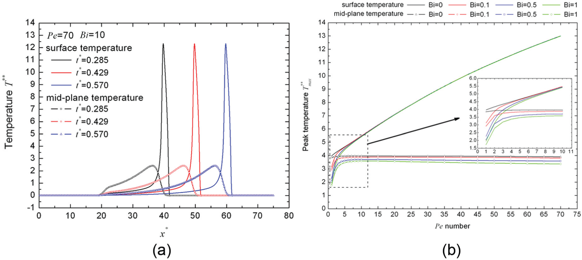
Corresponding to the steady states in Figure 4(c), the steady state temperatures at three instants with cooling effects are presented in Figure 9(a). Both the surface and mid-plane temperatures are decreased, and the “flat stage” no longer exists, while the peak surface temperature is still the same with that in the adiabatic situation. The evolutions of $T_{smax}^{* *}$ and the maximum mid-plane temperature $T_{mmax}^{* *}$ as function of Peclet number when d^* = 0.5 with several Biot values are shown in Figure 9(b) as well as the details of Pe < 10. When Bi = 0, $T_{smax}^{* *}$ increases linearly, which is the same as that shown in Figure 6(b), and $T_{mmax}^{* *}$ is kept at the “flat stage” level of 3.95. When Bi > 0 and Pe < 5, both $T_{smax}^{* *}$ and $T_{mmax}^{* *}$ decreased significantly, which means the convection has appreciable influences on them when the heat source is moving slowly. When Pe > 10, $T_{smax}^{* *}$ converges rapidly to the value of adiabatic situation (Bi = 0), and $T_{mmax}^{* *}$ rises to smaller constants. It tells that the cooling effects become insignificant and can be neglected with high moving speed.

Figure 9.

(a) Surface and mid-plane temperatures at three steady state instants when convection is applied and (b) variations of the peak surface and maximum mid-plane temperatures as function of Pe and Bi.

Conclusion and discussions

The transient heat transfer problem of finite thickness plate with moving heat source is investigated for the proper modeling of similar structures. The dependence of heat source intensity on the moving speed is considered with a new dimensionless temperature $T^{* *}$ which reflects the real temperature filed directly. The following conclusions are achieved:

1. With adiabatic boundary conditions, the steady state is quickly reached for fast moving heat source. The characteristic time has exponential relationship with the moving speed. The peak surface temperature of the plate exists in the contact area and increases linearly with the moving speed.

2. The plate thickness has great influences on the temperature field under symmetrically located moving heat sources. The peak surface temperature increases significantly when the dimensionless thickness d^* is thinner than the critical value for each moving speed. In this situation, the temperature field should be calculated with numerical methods instead of the analytical solutions of semi-infinite model. When d^* is thicker than the critical thickness, the peak surface temperature is not sensitive to the plate thickness. In this situation, the plate can be set up as a semi-infinite model, and the analytical solutions can be used for the temperature estimation around the contact area.

For commonly used disk brakes, the pads are usually longer than 80 mm, while the disk is thinner than 10 mm. The dimensionless thickness d ^* = 0.125 is thinner than the critical thickness even with high moving speed, and the surface temperature will be much higher than that calculated by the semi-infinite model, so the finite thickness model should be applied. For the pin-on-disk structures, d^* is usually larger than three. Even for slow moving, the disk still can be treated as semi-infinite model.

3. If the heat source moves slowly (Pe < 10), the cooling effects can decrease the surface and mid-plane temperatures significantly. On the opposite (Pe > 10), the cooling effects cannot make significant differences on the peak surface temperature in the contact area compared with that in the adiabatic situation, while they can decrease the mid-plane temperature. So for the modeling of practical structures, if the heat source is moving fast, although the convection is applied outside of the contact area, the peak surface temperature still can be evaluated by the adiabatic model. In this situation, although the body temperature is decreased, its non-uniformity in the sliding direction is enlarged. It may be more dangerous to the disk since local hot spots or surface cracks could happen.

Footnotes

Appendix 1

Academic Editor: Sang-Wook Kang

Declaration of conflicting interests

The author(s) declared no potential conflicts of interest with respect to the research, authorship, and/or publication of this article.

Funding

The author(s) disclosed receipt of the following financial support for the research, authorship, and/or publication of this article: This work is supported by the National Natural Science Foundation of China (No. 51175042 and No. 51575042) and Beijing Higher Education Young Elite Teacher Project (YETP1174).

References

Panier

Dufrénoy

Weichert

. An experimental investigation of hot spots in railway disc brakes. Wear 2004; 256: 764–773.

Lee

Barber

. Frictionally excited thermoelastic instability in automotive disk brakes. Journal of Tribology 1993; 115: 607–614.

Cristol-Bulthe

A-L

Desplanques

Degallaix

. Coupling between friction physical mechanisms and transient thermal phenomena involved in pad-disc contact during railway braking. Wear 2007; 263: 1230–1242.

. Thermal buckling of automotive brake discs. PhD Thesis, University of Michigan, Ann Arbor, MI, 2004.

Panier

Dufrénoy

Brunel

. Progressive waviness distortion: a new approach of hot spotting in disc brakes. J Therm Stresses 2005; 28: 47–62.

Day

. Investigation of disc/pad interface temperatures in friction braking. Wear 2007; 262: 505–513.

Meresse

Harmand

Siroux

. Experimental disc heat flux identification on a reduced scale braking system using the inverse heat conduction method. Appl Therm Eng 2012; 48: 202–210.

Jaeger

. Moving sources of heat and the temperature at sliding contacts. J Proc Roy Soc New S Wales 1942; 76: 203–224.

Tseng

M-L

Burton

. Thermal stress in a two-dimensional (plane stress) half-space for a moving heat input. Wear 1982; 79: 1–9.

10.

Laraqi

Alilat

Garcia

Maria

. Temperature and division of heat in a pin-on-disc frictional device-Exact analytical solution. Wear 2009; 266: 765–770.

11.

Yevtushenko

Kuciej

Yevtushenko

. Three-element model of frictional heating during braking with contact thermal resistance and time-dependent pressure. Int J Therm Sci 2011; 50: 1116–1124.

12.

Laraqi

Bairi

Segui

. Temperature and thermal resistance in frictional devices. Appl Therm Eng 2004; 24: 2567–2581.

13.

Aderghal

Loulou

Bouchoucha

. Analytical and numerical calculation of surface temperature and thermal constriction resistance in transient dynamic strip contact. Appl Therm Eng 2011; 31: 1527–1535.

14.

Yevtushenko

Grzes

. 3D FE model of frictional heating and wear with a mutual influence of the sliding velocity and temperature in a disc brake. Int Commun Heat Mass 2015; 62: 37–44.

15.

Belhocine

. Thermal analysis of a solid brake disc. Appl Therm Eng 2012; 32: 59–67.

16.

Adamowicz

Grzes

. Analysis of disc brake temperature distribution during single braking under non-axisymmetric load. Appl Therm Eng 2011; 31: 1003–1012.

17.

Choi

J-H

Lee

. Transient thermoelastic analysis of disk brakes in frictional contact. J Therm Stresses 2003; 26: 223–244.

18.

Zagrodzki

Lam

Al Bahkali

. Nonlinear transient behavior of a sliding system with frictionally excited thermoelastic instability. J Tribol: T ASME 2001; 123: 699–708.

19.

Carslaw

Jaeger

. Conduction of heat in solids. 2nd ed. London: Oxford University Press, 1959.

Modeling and analysis of transient temperature field in finite thickness plate under symmetrically located moving heat sources

Abstract

Keywords

Introduction

Model

Statement of the problem

Solution of the finite thickness model

Analytical solution of the semi-infinite model

Comparison of the solutions in semi-infinite model

Analysis of temperature field in the plate

Steady state

Temperature field with new dimensionless system

Influence of plate thickness and moving speed on the temperatures

Influence of convection on the temperature field

Conclusion and discussions

Footnotes

Appendix 1

Declaration of conflicting interests

Funding

References