Sage Journals: Discover world-class research

Abstract

Studies have shown that the structure of dolphin skin controls fluid media dynamically. Gaining inspiration from this phenomenon, a kind of bionic structural heterogeneous composite material was designed. The bionic structural heterogeneous composite material is composed of two materials: a rigid metal base layer with bionic structures and an elastic polymer surface layer with the corresponding mirror structures. The fluid control mechanism of the bionic structural heterogeneous composite material was investigated using a fluid–solid interaction method in ANSYS Workbench. The results indicated that the bionic structural heterogeneous composite material’s fluid control mechanism is its elastic deformation, which is caused by the coupling action between the elastic surface material and the bionic structure. This deformation can decrease the velocity gradient of the fluid boundary layer through changing the fluid–solid actual contact surface and reduce the frictional force. The bionic structural heterogeneous composite material can also absorb some energy through elastic deformation and avoid energy loss. The bionic structural heterogeneous composite material was applied to the impeller of a centrifugal pump in a contrast experiment, increasing the pump efficiency by 5% without changing the hydraulic model of the impeller. The development of this bionic structural heterogeneous composite material will be straightforward from an engineering point of view, and it will have valuable practical applications.

Keywords

Bionic structure heterogeneous composite material drag reduction efficiency enhancement

Introduction

The simulation of natural phenomena using the biomimetic approach is useful for addressing complex engineering problems and is an effective method for improving performance.^1–8 When an organism combines a number of factors such as morphology, structure and materials in a process known as biological coupling,^9,10 it improves abilities such as drag reduction,^11,12 noise reduction,^13,14 anti-adhesion¹⁵ and self-cleaning.^4,16 For example, there is a huge difference between the rapid swimming speed of a dolphin and the available physiological power needed to achieve that speed.¹⁷ The dolphin’s perfectly streamlined body is considered to be one of the main reasons for its speed,¹⁸ but many studies^19–22 have shown that the characteristics of the skin are also important. Matsumura et al.²³ found that wall deformation corresponds to an increase in the bulk mean velocity, as the deformation of the skin can only be observed when the dolphin swims rapidly, and wall deformation contributes to drag reduction by decreasing both the viscous shear stress and the Reynolds shear stress. Endo and Himeno²⁴ suggested that the typical shape of displacement of a compliant surface is a wave, which is almost homogeneous in the spanwise direction.

These studies consider only the elastic deformation of the dolphin’s epidermis and ignore the effect of the basal structure on that deformation. The objective of this study was thus to design a bionic structural material that fully takes into account both the elastic deformation of the dolphin’s epidermis and its basal structure. The new material comprises two different materials and is termed a bionic structural heterogeneous composite material (BSHCM). The fluid control mechanism of this BSHCM was investigated using a fluid–solid interaction simulation method and applied to a centrifugal pump impeller in a contrast experiment to determine its effect on pump efficiency.

Simulation conditions

Design of BSHCM

Dolphin skin has a specific bionic structure (see Figure 1(a)), with the epidermis exhibiting elasticity and the dermis having a certain hardness. These layers fit together through a particular structure and can control a fluid medium to reduce drag. Using the similarity principle, the structure of the BSHCM mimics that of dolphin skin after simplification, as shown in Figure 1(b). The surface material is a polymer with a certain elasticity, and the base contains metal materials with a certain hardness. The groove structure consists of two parts, one rectangular and one semicircular, seen in section view, that fit directly onto the base material. The parameters of the structure can be controlled by the length, depth and distance between the grooves. The length of the groove is R, the depth is H and the distance between them is D, as shown in Figure 1(c). The structures of the surface materials mirror those of the base, with D = D′, H = H′ and R = R′, where D′, H′ and R′ are the structural parameters of the surface material, as shown in Figure 1(d). The bionic structures of the two materials are thus engaged and may change slightly according to the application conditions. Under the action of fluid pressure, the BSHCM can control a fluid medium through the coupling action between the elasticity deformation of the surface material and the bionic structures of the basal metal material.

Figure 1.

Structure model of dolphin skin and the BSHCM: (a) schematic diagram of the structure of dolphin skin, (b) bionic structure of the mimicked dolphin skin model, (c) the parameters of the BSHCM and (d) the structure and parameters of surface material.

Simulation

Established simulation model

Pro/E software was used to establish the BSHCM model and an ordinary rigid smooth contrast (RSC) model. The structures and sizes of the two models are shown in Figure 2.

Figure 2.

The BSHCM and RSC models and their parameters: (a) structure of the BSHCM model, (b) parameters of the BSHCM model, front view, (c) structure of the RSC model and (d) parameters of the RSC model, front view.

Determination of the fluid domain

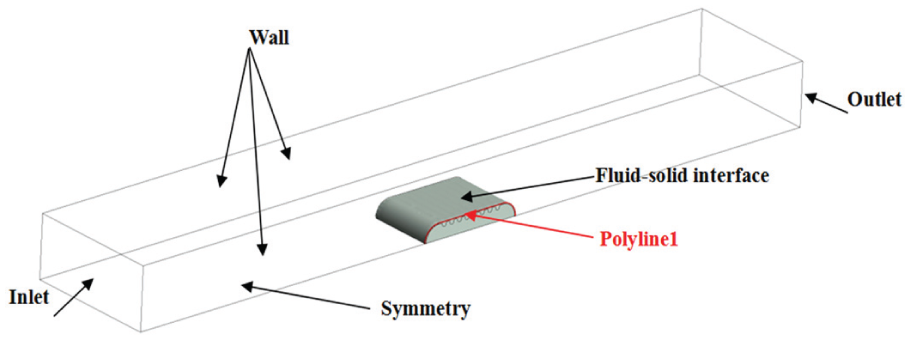
Based on the numerical simulation and the size of the simulation model, the computation domain is set as cuboids, as shown in Figure 3. The concrete size of the computational domain is 300 mm × 120 mm × 26.8 mm. The distance between the inlet and the front of the model is set as three times the length. The symmetry of the model allows for a half model to be used for numerical simulation and analysis. To analyse the different simulation results of the models, a curve intersected by the symmetry surface and the fluid–solid interface is defined, named polyline1 (Figure 3).

Figure 3.

Computed field applied in the numerical simulation.

Discrimination of the computation domain

The main concerns with the BSHCM are coupling deformation and stress in the fluid–structure coupling process. Mesh quality is the key factor determining whether the coupling calculation can be made; in this study, the tetrahedron elements are used both for the fluid and solid domains, with the near-wall grid densified using the size functional method. This guarantees the calculation accuracy and saves calculation time. A grid independence study performed with BSHCM model (stream flow speed = 5 m/s) is shown in Table 1; when the grid number achieved 2 million, it was found that the calculation results did not change depending on it. The mesh of Yplus on the solid model and final grids are shown in Figure 4(a)–(c).

Table 1.

Grid independence study.

Plan	Grid no.	Viscous drag (N)	Pressure drag (N)	Total drag (N)
1	8 × 10⁵	0.6136	0.1040	0.7824
2	1.5 × 10⁶	0.6874	0.1284	0.8287
3	2 × 10⁷	0.6988	0.1304	0.8292
4	2.5 × 10⁷	0.6997	0.1311	0.8294

Figure 4.

Grids of the BSHCM: (a) Yplus distribution on the fluid–solid interface, (b) grid map on the symmetry plane and (c) local solid domain grids.

Two-way fluid–solid interface (FSI) platform

A two-way coupled computational platform was established using the ANSYS Workbench 14.0 software, and its calculation principle is shown in Figure 5. The solution requires two separate solvers, one for the fluid (CFX 14.0) and the other for the structure (Transient structural 14.0), which run in sequential order with synchronisation points to exchange information at the interface.^25,26 The core of the two-way fluid-solid interaction simulation is the force of the fluid domain and the displacement of the structure domain, resulting in constant transfer through the fluid–solid interface. The key step is thus the setting of the FSI.²⁷

Figure 5.

Calculation principle process based on Workbench.

Turbulent model, material parameters and boundary conditions

In this study, standard $k - ε$ is adopted after considering the multi-precision calculations and computation time. According to the turbulent viscosity hypothesis of Boussinesq,²⁸ the Reynolds stress can be expressed as

- ρ \bar{{u'}_{i} {u'}_{j}} = μ_{t} (\frac{\partial u_{i}}{\partial x_{j}} + \frac{\partial u_{j}}{\partial x_{i}}) - \frac{2}{3} δ_{ij} (ρ k + μ_{t} \frac{\partial u_{j}}{\partial x_{i}})

(1)

where δ_ij is the Kronecker delta, u_i is the fluctuating velocity, µ_t represents the turbulent eddy viscosity and $K = 1 / 2 \bar{{u'}_{i} {u'}_{j}}$ is the turbulent kinetic energy.

From the foregoing formula, the governing equations of turbulent kinetic energy K and dissipation rate ε are expressed as equations (2) and (3), respectively

\frac{\partial (ρ k)}{\partial t} + \frac{\partial (ρ u_{i} k)}{\partial x_{i}} = \frac{\partial}{\partial x_{j}} [(μ + \frac{μ_{t}}{σ_{k}}) \frac{\partial k}{\partial x_{i}}] + ρ (P_{k} - ε)

(2)

\frac{\partial (ρ ε)}{\partial t} + \frac{\partial (ρ u_{i} ε)}{\partial x_{i}} = \frac{\partial}{\partial x_{j}} [(μ + \frac{μ_{t}}{σ_{ε}}) \frac{\partial ε}{\partial x_{i}}] + ρ \frac{ε}{k} (C_{1} P_{k} - C_{2} ε)

(3)

where µ is the molecular viscosity coefficient, u_i represents the velocity component in the corresponding direction, ρ is the fluid density, C_µ are the constants of the turbulence model and P_k is the generation term of turbulent kinetic energy, which can be defined as in equation (4). The constant values of the model are C_µ = 0.09, C₁ = 1.44, C₂ = 1.92, σ_k = 1.0 and σ_ε = 1.3

P_{k} = \frac{μ_{t}}{ρ} (\frac{\partial u_{i}}{\partial x_{j}} + \frac{\partial u_{j}}{\partial x_{i}}) \frac{\partial u_{i}}{\partial x_{j}}

(4)

The inlet was set as the velocity boundary, with the velocity and turbulence intensities set as 5 m/s and 0.5%, respectively. The outlet was set as a constant pressure boundary with a static pressure of 0 Pa. The model’s middle surface was set as symmetry. A nonslip, smooth wall was applied at the interface and other surfaces. Based on the platform, the displacement results and the force results in the solid and fluid domains were transmitted and calculated through the FSI. Two parameters have important effects on the fluid medium, namely, the elasticity modulus of the surface material (see Table 2) and the groove distance (see ‘d’ in Figure 2(b), d = 2, 3 and 4 mm were selected, respectively). The transient calculation is used in this study. In the process of bidirectional fluid–structure coupling calculation, the time step was set as 0.01 s, the iteration number of each step is range from 3 to 10 and the convergence criteria for all points were set at 10⁻⁵ root mean square (RMS). All the content has been added and highlighted in the article. The material properties of the solid domain are shown in Table 2.

Table 2.

Physical property of material.

Material	Density (kg/m³)	Elasticity modulus (Pa)	Poisson’s ratio
Basal material	7850	2 × 10¹¹	0.3
Surface material	1300	5 × 10⁶	0.48

Results and discussion

Verification of the accuracy of the simulation results

Figure 6(a) and (b) gives the trends of the velocity and turbulent kinetic energy of polyline1 at different velocities. As the fluid velocity increases, the trend of the polyline1 of the BSHCM changes accordingly (see Figure 6(a)). The turbulent kinetic energy is in proportion to the velocity, as in the formula $K = 1 / 2 \bar{{u'}_{i} {u'}_{j}}$ , so the trend should be consistent with that of the velocity. Figure 6(b) confirms this and indicates that the results of the simulation are empirical and plausible.

Figure 6.

Trend of the velocity and turbulent kinetic energy: (a) velocity on polyline1 and (b) turbulent kinetic energy on polyline1.

Effect of the BSHCM on the interface velocity

Figure 7(a) and (b) gives the FSI contour of the BSHCM and RSC models when the stream flow speed is 5 m/s. In theory, in the no-slip condition, the speed at the FSI is 0,²⁹ so the FSI velocity of the BSHCM should be 0, as in the RSC model (see Figure 7(b)). This is not the case in practice, and the velocity of the BSHCM takes on an uneven distribution (Figure 7(a)). For the RSC model, the fluid–solid interface (FSI) coincides with the fluid–solid actual contact surface (ACS), as shown in Figure 8(a). The surface velocity at the FSI is thus 0 when the fluid is flowing along it. For the BSHCM model, however, under the action of fluid pressure, the position of the ACS is lower than that of the FSI because of the coupling deformation between the elastic surface material and the bionic structures of the basal material (see Figure 8(b)). In this condition, the FSI is no longer consistent with the ACS. The velocity at the position of O on the FSI is thus not 0, but is $u_{i}$ and $u'_{i}$ , respectively. This is why the velocity of the FSI is not 0 and the distribution is uneven.

Figure 7.

Contour of the interfacial velocity: (a) fluid–solid interface (FSI) of the BSHCM and (b) fluid–solid interface (FSI) of the RSC.

Figure 8.

Schematic diagram of the velocity gradient: (a) velocity gradient of the RSC model and (b) velocity gradient of the BSHCM.

Figure 8(a) and (b) indicates that in the boundary layer, the velocity gradient of the BSHCM is smaller than that of the RSC model. As previously seen, the frictional force of the boundary layer can be expressed as $F = μ A (du / dy)$ , where µ is the dynamic viscosity of the fluid, A is the contact area and $du / dy$ is the velocity gradient. Because the pressure force caused by micro-elastic material deformation is much smaller than fractional force, so it can be inferred that the fractional force of the BSHCM model is smaller than that of the RSC model.

From the foregoing results and analysis, it can be deduced that the BSHCM has the function of drag reduction, achieved by a decreasing velocity gradient through elastic deformation.

Effect of the BSHCM on the turbulent kinetic energy

Figure 9 shows the turbulent kinetic energy curves of the BSHCM and RSC models at a velocity of 5 m/s, from which it can be seen that the shape of the turbulent kinetic energy of the two models is like an asymmetric saddle. The turbulent kinetic energy of the BSHCM model is obviously lower than that of the RSC, particularly when the fluid is immediately in contact with the model. This indicates that the energy dissipation of the BSHCM is lower than that of the RSC model. When water flows through the surface of the RSC, the overcoming of resistance by the fluid is compensated by the mechanical energy of the fluid itself. This portion of energy is permanently transformed into heat energy and dissipates. However, when the water flows through the surface of the BSHCM, some displacement and deformation are produced because of the elastic surface material coupled with the bionic structures. Part of the energy is thus transformed into elastic potential energy and stored by elastic deformation. During the process of restoring the deformation, at a particular point the elastic potential energy is transformed into kinetic energy. This indicates that in the BSHCM model, only part of the energy is transformed into heat energy, so the energy dissipation of the model is lower than that of the RSC model.

Figure 9.

Turbulence kinetic energy of the RSC and BSHCM models at u₀ = 5 m/s.

From the foregoing analysis, it follows that the BSHCM model can absorb part of the energy through elastic deformation, effectively reducing the turbulent kinetic energy, avoiding excessive exchange at the FSI and thus energy loss.

Fluid control mechanism of the BSHCM

Figure 10(a) shows a schematic of the displacement changes in the BSHCM and RSC models at a velocity of 5 m/s, illustrated with a double y. The right side of the blue Y-axis represents the displacement value of the RSC model, while the left side of the black axis is that of the BSHCM model. Figure 10(a) shows that the displacement of the BSHCM is much larger than that of the RSC model, indicating that the former has obvious deformation (also seen in Figure 10(b)). The displacement of the BSHCM shows that the deformation is very regular and can be divided into three parts: A, B and C. Parts A and C are the elastic material coupled with the rigid smooth basal material, while B is the elastic material coupled with the rigid bionic structure basal material. The displacement of A and C takes on wavelike changes. When the unstable flow meets the elastic surface material, periodic waves similar to a Tollmien–Schlichting wave (T-S wave)³⁰ are generated, with wave lengths of λ₁ and λ₃, respectively, and these have a close relationship in front of the flow. The fluid situations of A and C illustrate the passive adaptability to the fluid dynamic response. However, part B can actively control the fluid, as the wavelength λ₂ can be controlled by the bionic structure size of the basal material, obtained by optimising certain parameters of the BSHCM, such as the elastic modulus, the thickness of the surface material and the structure size of the basal material. Thus, the key factor in the fluid control mechanism of the BSHCM is the deformation caused by the coupling action between the elastic surface material and the bionic structure.

Figure 10.

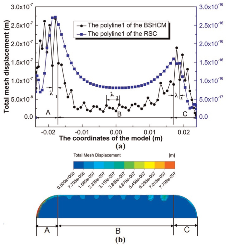
Schematic diagram of the total deformation: (a) graph of the node displacement on the polyline1 and (b) total displacement of the BSHCM.

Effect of BSHCM on pump efficiency: a simple contrast experiment

This section describes the application of the BSHCM in the impeller of a 200QJ50-26 centrifugal pump to investigate its effect on efficiency.

Test description

The realisation of the BSHCM on the impeller comprised two steps. First, the bionic structures were realised on the basal material. The cast iron of the impeller was used as the basal material and cast bionic structures were applied to the impeller directly, using a special casting method.³¹ Because the groove geometry is not the key factor to influence the fluid flow³² and the difficulty of processing, a riblet form of bionic structure was used, with a regular triangle section form (see Figure 11(a)). The parameters of the riblet were L = 0.5 mm, D = 2 L mm and H = 0.866 L mm. The riblet form cast on the impeller is shown in Figure 11(b). Second, an elastic surface material was composited on the basal bionic structures. Polyurethane (PU) (with a hardness value of shore A50) was used as the surface coating material. The PU obtained by the polyurethane prepolymer (PUP) (with the molecular formula C10H8N2O2 C6H14O3) was mixed with a curing agent (with the molecular formula C13H12N2CL2) according to the mass ratio 100:12. The impeller with the bionic structure was dipped into the PU mixture and then rotated at a specific speed until the PU mixture solidified. A thin and elastic PU surface layer firmly coated the basal bionic structure. The impeller with the attached BSHCM was then vulcanised in a vulcanising machine. The initial vulcanising temperature was 120°C, and the duration 15 min. To prevent wearing, the attachment of the BSHCM to the impeller required a second vulcanisation at 100°C for 8 h. The impeller is a bionic impeller, as shown in Figure 11(c), and the pump, assembled from two bionic impellers, is termed a bionic pump, as shown in Figure 11(d).

Figure 11.

Realisation process of the BSHCM in the sample: (a) physical model of the bionic structure, (b) bionic structure cast on the complex channel of the pump impeller, (c) impeller with the BSHCM and (d) bionic pump.

Experimental method and facility

Following the aforementioned process, 18 bionic impellers were processed and 9 bionic pumps assembled. Repeatability and contrast tests were carried out on the bionic pumps (the channel of impeller coated with BSHCM) and on ordinary water pumps to investigate the effect of the BSHCM on efficiency. To avoid the effect of different engines on the efficiency of the pumps during the contrast experiment, two kinds of engine were used. Samples 1 and 2 were from ordinary water pumps (the channel of impeller is cast iron); samples 3, 4, 5, 6 and 7 were from bionic pumps with the same type of engine as the ordinary pumps and samples 8, 9, 10 and 11 were from bionic pumps with different engine types from the ordinary pumps.

Another two ordinary pumps coated with PU, which has the same properties as the BSHCM surface material, were selected as contrast samples to observe the improvement associated with the BSHCM. Samples 12 and 13 are from the PU pumps.

The performance tests were carried out on the diving pump test bed shown in Figure 13. The tested impeller was installed in the pump casing. The flow capacity and pressure were detected by a flow sensor and pressure sensor. These are extremely accurate sensors (within 0.05%) and can be controlled by the flow control valve. The testing signal input to the pump was through an integrated automatic test system. The pump performance parameters were obtained with the data processing system.

The experimental set-up shown in Figure 12 has the following parts: (1) an electric engine used to drive the pump and (2) a centrifugal pump used for the experiment. These include the following: (3) a pressure pipeline, (4) a pressure sensor, (5) a speed discrepancy meter, (6) a LWGY-type turbine flow sensor used to examine the pressure and speed of the water, (7) a flow control valve used to control the flow capacity, (8) a PMS-integrated automatic test system and (9) a data processing system for data collection and processing.

Figure 12.

Sketch of the diving pump test bed.

Experimental results and analysis

Figure 13 shows the relationships between the efficiency and pump capacity of all the pumps. From Figure 13(a), it can be seen the efficiency levels of all bionic pump samples were higher than those of the ordinary pumps, particularly at an effective work range of 40–65 m³/h (the effective work range of the 200QJ50-26 water centrifugal pump is between 40 and 65 m³/h). The highest observed efficiency for the ordinary pumps was about 69%, which occurred at a pump capacity of 55 m³/h. Above this level, the efficiency decreased dramatically. In contrast, the highest efficiencies (74%–75%) for most of the bionic pumps occurred in the pump capacity range of 55–60 m³/h. The efficiency enhancement of the bionic pumps was about 5%. After this point, the efficiency slowly decreased. The effective curves for all the bionic pumps became more compressed. In the effective work range, the bionic pumps could thus work continuously at a higher efficiency level. The efficiency enhancement of the bionic pumps was also stable (it has no relationship with the engine). Figure 13(b) shows the flow–efficiency relationships of the bionic, ordinary and PU pumps. Although the efficiency of the PU pumps is higher than that of the ordinary pumps, it is still much lower than that of the bionic pumps. That is, although the PU is coated on the polished surface of the ordinary pumps, when it couples with the groove structures on the basal material the pumps are able to control the fluid medium dynamically as shown in section ‘Results and discussion’. The experimental results indicate that the BSHCM enhanced the efficiency of the pumps.

Figure 13.

Flow–efficiency relationships of all pumps: (a) the bionic and the ordinary pumps and (b) the bionic, the ordinary and the PU pumps.

With the increased flow capacity, the pumps head decreased dramatically, as shown in Figure 14. However, the trends of pump head among the pumps are almost the same, that means the pump head are not affected by the BSHCM. As we know, the pump efficiency η can be expressed as follows

η = \frac{ρ g Q H}{P} \times 100 %

(5)

where Q is the pump capacity (m³/h), H is the pump head (m), ρ refers to the density of the fluid medium (kg/m³) and P refers to the shaft power (kg m/s). From Figure 13, we can see that the pump efficiency of bionic pump is enhanced while the pump head is not affected almost (see in Figure 14), that means the shaft power of the bionic pump will decrease, that is to say, the pump power decreases. The above analysis means that the BSHCM not only improves the pump efficiency but also decreases the pump shaft power and so saves the energy.

Figure 14.

Flow–head relationship of all pumps.

Conclusion

The findings presented in this article indicate that the BSHCM’s active fluid control reduces drag and enhances pump efficiency. The core of that control is the coupling deformation between the elastic surface material and the bionic structures of the basal material. Hence, there are two aspects of the BSHCM’s fluid control mechanism. First, as the deformation pushes the fluid–solid ACS downward, the velocity gradient of the fluid boundary layer decreases, resulting in frictional force reduction. Second, the elastic deformation absorbs some of the energy, effectively reducing the turbulent kinetic energy, avoiding excessive exchange and energy loss at the fluid–solid interface.

Footnotes

Academic Editor: Duc T Pham

Declaration of conflicting interests

The author(s) declared no potential conflicts of interest with respect to the research, authorship and/or publication of this article.

Funding

The author(s) disclosed receipt of the following financial support for the research, authorship and/or publication of this article: The authors are grateful for the grants received from the National Natural Science Foundation of China (grant no. 51475203), the Science and Technology Development Project of Jilin Province (grant no. 20140307030GX) and the Changchun special project of major scientific research (grant no. 13KG33).

References

Fish

FE.

Biomimetics: determining engineering opportunities from nature. Bioinspir Biomim 2009; 7401: 740109.

Favier

Pinelli

Piomelli

Control of the separated flow around an airfoil using a wavy leading edge inspired by humpback whale flippers. CR Mecanique 2012; 340: 107–114.

Wong

Kang

Tang

SKY

. Bioinspired self-repairing slippery surfaces with pressure-stable omniphobicity. Nature 2011; 477: 443–447.

Ebert

Bhushan

Durable lotus-effect surfaces with hierarchical structure using micro-and nanosized hydrophobic silica particles. J Colloid Interf Sci 2012; 368: 584–591.

Fish

Weber

Murray

. The tubercles on Humpback whales’ flippers: application of bio-inspired technology. Integr Comp Biol 2011; 51: 203–213.

Fish

Howle

Murray

MM.

Hydrodynamic flow control in marine mammals. Integr Comp Biol 2008; 48: 788–800.

Tuteja

Choi

. Designing superoleophobic surfaces. Science 2007; 318: 1618–1622.

Kundu

SC.

Bio-inspired fabrication of fibroin cryogels from the muga silkworm Antheraea assamensis for liver tissue engineering. Biomed Mater 2013; 8: 055003

Ren

Liang

YH.

Biological couplings: function, characteristics and implementation mode. Sci China Technol Sc 2010; 53: 379–387.

10.

Ren

Liang

YH.

Preliminary studies on the basic factors of bionics. Sci China Technol Sc 2014; 57: 520–530.

11.

Tian

Ren

L-q

Liu

Q-p

. The mechanism of drag reduction around bodies of revolution using bionic non-smooth surfaces. J Bionic Eng 2007; 4: 109–116.

12.

Wang

JM.

Experimental study of the drag reduction and separation efficiency for a new hydrocyclone with a Reducing Pressure Drop Stick. Mater Design 2012; 98: 7–15.

13.

Chen

Liu

Liao

. The sound suppression characteristics of wing feather of owl (Bubo bubo). J Bionic Eng 2012; 9: 192–199.

14.

Shi

Zhang

Wang

. Numerical simulation of the effect of bionic serrated structures on the aerodynamic noise of a circular. Bionic Eng 2012; 9: 91–98.

15.

Ren

LQ.

Progress in the bionic study on anti-adhesion and resistance reduction of terrain machines. Sci China Ser E 2009; 52: 273–284.

16.

Barthlott

Neinhuis

Purity of the sacred lotus, or escape from contamination in biological surfaces. Planta 1997; 202: 1–8.

17.

Pavlov

VV.

Dolphin skin as a natural anisotropic compliant wall. Bioinspir Biomim 2006; 1: 31–40.

18.

Fish

FE.

The myth and reality of Gray’s paradox: implication of dolphin drag reduction for technology. Bioinspir Biomim 2006; 1: R17–R25.

19.

Nagamine

Yamahata

Hagiwara

. Turbulence modification by compliant skin and strata-corneas desquamation of a swimming dolphin. J Turbul 2004; 5: 1–25.

20.

Kramer

MO.

Boundary layer stabilization by distributed damping. J Am Soc Nav Eng 1960; 72(1): 25–34.

21.

Takashima

Koyama

Hagiwara

Direct numerical simulation on turbulent flow around a regularly deforming film. Adv Turbul 2007; 117: 662–664.

22.

Carpenter

Davies

Lucey

AD.

Hydrodynamics and compliant walls: does the dolphin have a secret. Curr SCI India 2000; 79758–765.

23.

Matsumura

Koyama

Hagiwara

Turbulent drag reduction by wall deformation synchronized with flow acceleration. IUTAM Symp Comput Phys New Perspect Turbul 2008; 4: 385–390.

24.

Endo

Himeno

Direct numerical simulation of turbulent flow over a compliant surface. J Turbul 2002; 3: 7–11.

25.

Gursul

Cleaver

Wang

Control of low Reynolds number flows by means of fluid–structure interactions. Mater Design 2014; 6417–55.

26.

Nakata

Liu

A fluid–structure interaction model of insect flight with flexible wings. J Comput Phys 2012; 231: 1822–1847.

27.

Klammer

Numerical analysis and characterization of bionic valves for microfluidic PDMS-based systems. J Micromech Microeng 2007: 17: s122–s127.

28.

Launder

Spalding

DB.

The numerical computation of turbulent flows. Comput Method Appl M 1974; 3: 269–289.

29.

Day

MA.

The no-slip condition of fluid dynamics. Erkenntnis 1990; 33: 285–296.

30.

Visbal

Gordnier

RE.

Numerical simulation of the interaction of a transitional boundary layer with a 2-D flexible panel in the subsonic regime. J Fluid Struct 2004; 19: 881–903.

31.

Tian

Chen

. Casting method of rib-like bionic non-smooth surface. T Chin Soc Eng Agr 2011; 27: 189–194.

32.

Qingping

Binary bionic coupling research on water-solid interface system for drag reduction. Doctoral Dissertation, Jilin University, Changchun, China, 2013.

The fluid control mechanism of bionic structural heterogeneous composite materials and its potential application in enhancing pump efficiency

Abstract

Keywords

Introduction

Simulation conditions

Design of BSHCM

Simulation

Established simulation model

Determination of the fluid domain

Discrimination of the computation domain

Two-way fluid–solid interface (FSI) platform

Turbulent model, material parameters and boundary conditions

Results and discussion

Verification of the accuracy of the simulation results

Effect of the BSHCM on the interface velocity

Effect of the BSHCM on the turbulent kinetic energy

Fluid control mechanism of the BSHCM

Effect of BSHCM on pump efficiency: a simple contrast experiment

Test description

Experimental method and facility

Experimental results and analysis

Conclusion

Footnotes

Declaration of conflicting interests

Funding

References