
Abstract
In this article, a new method is proposed to help the mobile robot to avoid many kinds of collisions effectively, which combined past experience with modified artificial potential field method. In the process of the actual global obstacle avoidance, system will invoke case-based reasoning algorithm using its past experience to achieve obstacle avoidance when obstacles are recognized as known type; otherwise, it will invoke the modified artificial potential field method to solve the current problem and the new case will also be retained into the case base. In case-based reasoning, we innovatively consider that all the complex obstacles are retrieved by two kinds of basic build-in obstacle models (linear obstacle and angle-type obstacle). Our proposed experience mixing with modified artificial potential field method algorithm has been simulated in MATLAB and implemented on actual mobile robot platform successfully. The result shows that the proposed method is applicable to the dynamic real-time obstacle avoidance under unknown and unstructured environment and greatly improved the performances of robot path planning not only to reduce the time consumption but also to shorten the moving distance.
Introduction
During the past two decade, robotics has been developed rapidly. Many researchers put their attentions on the navigation of mobile robots. The most basic technology of navigation is path planning which is going to find a safe and efficient way from starting point to target. In recent years, research on path planning has focused on local searching in dynamic environments, where the pose and location of the obstacles are unknown or partially unknown.
A well-known approach to localize the path of mobile robots is artificial potential field (APF) method, 1 which is used commonly in real-time collision avoidance and smooth path for mobile robots because of its elegant mathematical analysis and simplicity. However, its inherent defects are obvious. First, Robot cannot reach the target nearby the obstacle. The obstacle repulsion increases and gravity decreases rapidly when target point is within the influence scope of obstacle. Second, there is a local minimum problem; when robot is in the process of traveling, the direction of total force and the movement direction of planning path are on the same straight line, and robot cannot avoid obstacle effectively but vibrates back and forth in a certain range. A lot of researchers have proposed some improvements on the traditional APF method in recent years. In 2003, MC Lee and Park 2 proposed an improved APF method using a virtual obstacle concept. A virtual obstacle is located around local minimums to repel the mobile robot. This method is adaptable for a real-time path planning because of its lower complexity. However, it is not suitable for the discrete modeling of the mobile robot in complex situation. In 2009, S Charifa and Bikdash 3 presented an adaptive boundary following algorithm guided by APF to avoid the local minima. When the size of obstacles is large, too much computing time need to be taken to guide the robot. In 2011, Q Li et al. 4 improved the APF method by providing an additional force and developing the virtual local minimum. The genetic algorithm was introduced to optimize the parameters such as the revolved angle of repulsion. The proposed method could plan out a simple, smooth, and safe path by simulation experiments, but not be applicable to the real world. In 2012, L Guan-chen et al. 5 integrated APF approach with receding horizon control method. An additional control term was added in path planning to escape from local minima of APF. This term accomplishes the description of specified property index except for distance and control energy, but the computational process is complicated. In the same year, Q Song and Liu 6 presented a dynamic fuzzy APF method to overcome the shortcomings of APF method. Through taking the advantage of velocity vector, modifying the potential field force function, and integrating with the fuzzy control method, all those steps could achieve adjusting the factors of repulsion potential field in real time. However, inputting the fuzzy control method increases the planning time greatly, and in practical applications, the impact of acceleration should be considered.
Moreover, several artificial intelligence algorithms such as fuzzy logic, 7 neural networks, 8 and genetic algorithm 9 have been proposed for the mobile robot navigation problem in unknown environments. The varied information of the environment needs to be detected by sensors to help the robot avoid obstacles autonomously. Those algorithms could achieve optimal local path planning, but they are relatively complex, time-consuming, and not very useful for real-time applications.
In fact, one of the main issues for mobile robot to navigate in uncertain environment is the lack of prior information. If environmental information could be acquired before path planning, it would contribute to guide the robot moving from the starting point to the target. Case-based reasoning (CBR) 10 is a technique that can reuse previous experience to obtain the suitable information to solve the current problems. Actually, CBR has been used in robotics to perform different tasks for many years. In 2003, Kruusmaa 11 presents a global navigation strategy for autonomous mobile robots in dynamic environments. CBR is used to store those solutions and their outcomes for a later use. It can improve the performance of the robot in a difficult uncertain environment, while is not efficient in simple dynamic environments. Moreover, the restrictions of this approach are that the size of the environment and the position of the goal points have to be known precisely, and the localization errors have to be small (just like it is with outdoor applications with global positioning system (GPS)). Urdiales et al. 12 in 2006 proposed a sonar-based purely reactive navigation technique for mobile platforms which was relied on CBR algorithm. CBR is used here to let a robot learn how to react in any given situation, so that it can adapt itself to any configuration or environment. However, this system is a purely reactive scheme, its case base can only be trained and learnt by human intervention or other high-level planner system in advance to realize autonomous path planning and does not have the ability to self-learning by its own build-in basic case base. Hodál and Dvořák 13 in 2008 combined CBR with graph algorithms, which is represented by a rectangular grid. It is applicable to the large-scale environments, saving computing time and traveling distance; nevertheless, the process is too complex to reduce the efficiency of the algorithm. To sum up, CBR technique can improve the performance of path planning for mobile robots in complicated environments, while the efficiency and applicability are different when CBR has been used in different platforms.
In this article, we proposed a new method which combines CBR method with the modified artificial potential field method (MAPF); we call it “EMMAPF” (experience mixing with modified artificial potential field method). In CBR, we innovatively consider that all the complex obstacles are retrieved by two kinds of basic build-in obstacle models (linear obstacle and angle-type obstacle). Meantime, the self-learning process also stores the past experiences into case base to rapidly generate an effective solution to solve the current problem in path planning when similar situations exist. “MAPF” method is utilized as a basic method to offer basic paths for the case base. 14 No matter in simple situations or in complicated environments, this method always guides the robot with an optimal path. In section “‘EMMAPF’ method,” a detailed description of “EMMAPF” method is represented, including the modified APF method and CBR technique. In section “Experiment,” we tested our algorithm on a mobile robot by simulating in MATLAB and real test in physical environment. Finally, we summarize the conclusion and future plan.
“EMMAPF” method
In this section, a detailed description of “EMMAPF” method is represented, including the modified APF method and CBR technique. By retrieving and adapting past problems from the case base, we can obtain the solution for current problem; this method can not only help the robot to avoid the obstacles autonomously but also save the computing time and traveling distance to obtain an optimal path.
The procedure of “EMMAPF” method is shown as above (Algorithm 1).
“EMMAPF” algorithm.

When the existence of obstacles around the robot is detected by sensors, some related information would be returned to system. After sorting and calculation, it will retrieve the similar cases from the case base based on those attribute datum. If the returned solutions are more than one, select the closest case, and then reset the transferring direction. Otherwise, the system will invoke the “MAPF” method. Finally, evaluate the proposed solution by the cost r(Pp) and update the system by learning from the case base. Thus, in CBR system, learning and adaptation are through accumulation of cases.
“MAPF” method
The traditional APF method is commonly used in real-time obstacle avoidance and smooth path for mobile robots. It is particularly attractive because of its elegant mathematical analysis and simplicity. However, there exists a local minima problem, and no optimization process is involved. Liu et al. 15 have proposed a concept of virtual obstacle to solve this problem. The virtual obstacle is located around local minimums to repel the mobile robot. We make some improvements based on this approach, modify the potential field force function, and set the virtual obstacle according to the shapes of obstacles detected by the sensor. The steps are shown as follows.
Modify the potential field force function
The attractive force function is described in formula (1)

where
The repulsive force functions are described in formulas (2)–(5)

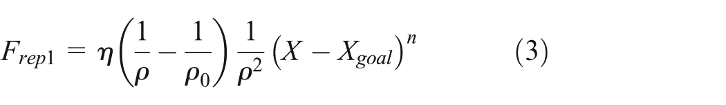

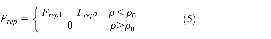
where
The total force is described in formula (6)

where
Set the virtual potential field area
While the robot gets trapped in a local minimum, it will stop there or repeat the same route back and forth in a certain range. There are two cases of local minimum shown in Figure 1.

Two cases of local minimum: (a) local minimum case 1 and (b) local minimum case 2.
In 2009, Dr Lei 16 proposed a new method which increases a special virtual potential based on the original repulsion field to solve this problem. They used a combination method to push the robot away from the local minima. Based on this method, we set the virtual potential field area as the shaded part in Figure 2. When the robot encounters the local minima, take the target point as the center, and calculate the radius R by equation (7) as the virtual potential field area

where

“MAPF” method to solve the local minimum: (a) local minimum case 1 and (b) local minimum case 2.
CBR technique
CBR is a self-learning method which helps to solve the current problem by re-using past cases and experiences to adapt to the changes in the environment. This method is based on the concept that similar problems have similar solutions. The innovation of our proposed CBR algorithm is that the cases of complex obstacles can be retrieved by two basic build-in case models which composed of “linear obstacle model” and “angle-type obstacle model.” Three steps can represent a simplified description of our CBR technique: retrieving the most similar case or cases, revising the proposed solution, and learning and retaining the new case for future problem solving. The flowchart of CBR technique is shown in Figure 3.

Flowchart of CBR technique.
Case representation
When using CBR technique to achieve path planning for mobile robots, the first fundamental decision to be made is how to establish a case base. Cases can be stored in many different representational formats, 17 such as framework representation, object-oriented representation, and predicate representation. Because of its features of applicability, summarizing, structuring, and reasoning, we choose framework as the representational format. A classical case base usually includes characteristic of the problem and the relevant solution that was used on an earlier occasion when a similar situation was encountered. A case can be described as follows


where

where
caseID: identifier of the obstacle;
obstacleCategory: the category of the obstacle’s front shape where the sensor could scan, such as line, convex polygon, concave polygon, and so on;
leftDistance/rightDistance: the length of the obstacle. If the obstacle category is linear, rightDistance will be set as zero;
angle: the global angle of the obstacle/the angle between two sides. Angle ranges between 0 and π;
rightAngle: the global angle of the right border. rightAngle ranges between 0 and 2*π. While the obstacle category is linear, rightAngle will be set as zero;
flag: each situation has two transferring direction, flag = 0 represents the direction of right, flag = 1 represents the left direction, flag describes which direction would be better for the current situation

resetDirection: the transferring direction for the robot.
If the obstacle category is linear, the function of the transferring direction is as follows

Else, if the obstacle category is angle-type, such as convex obstacle or concave obstacle, the transferring direction is

Method of representing case base on Extensible Markup Language
Extensible Markup Language (XML) is a user-defined markup language, which is a set of specifications created by World Wide Web Consortium (W3C) and designed to transport and store data. It is a new generation of web language that uses tree structure, adapts for multi-subsystem architecture in case base, and would be able to describe the relationship between the data.
XML language has good data storage format, is high-structured, and is easy for network transmission, compared with traditional relational databases; the expansibility and reusability of XML are better.
CBR is an incremental and sustainable self-learning process. For retrieving and re-using the previous case, it needs to constantly update the case base. Using XML technology to establish a CBR case-base system has the following advantages:
Due to a unified data format, standard XML supports the exchange of data between different data sources, so the system can solve the same case in different areas of shared problems, to achieve distributed storage and retrieval of cases.
XML processing can be independent of the data, so the case can be handled by the other XML applications and also easy to restructure the flow of information between the CBR system and other systems.
There are three aspects to indicate the case:
Case category: to classify case and build index, be convenience for retrieving;
Case character: it is used to describe character of the case, distinguish the differences between cases;
Case solution: make out the solution for the cases.
Empirical formulas
Our Robot is a three omni-wheel mobile robot. We set the simulation model based on iRobot Open Source project. In simulation environment, complex obstacle is constituted by two kinds of basic obstacle models; the empirical formulas are described as below.
Linear-type obstacle
In the open source project of iRobot, obstacle is represented by
If the type of obstacle is linear, each parameter value of the obstacle in case base is described as below:
where
When the robot encounters a linear obstacle, the direction of movement is determined as follows


where
Deflection angle formula is shown in equation (12). It is a kind of way to walk along the wall when robot encounters a linear obstacle.
Angle-type obstacle
Similarly, angle-type obstacle is composed of two walls with one angle.
Each parameter value of the obstacle in case base is described as below:


Here, the point of intersection will be replaced with
If
When the robot is contacting with the corner of the two walls, there are two scenarios need to be considered, that is, whether to do circular motion around the corner or directly flee away. The velocity vector is decomposed into two orthogonal components. One component along with the line from the corner to the robot. If the intended velocity of the robot has a component directed from the corner to the robot, then it will drive away directly. The other situation is when the component is directed from robot to the corner, the robot will do a circular motion around the corner. The radius of the circular motion is set equal to the radius for avoiding the obstacle.
The other complex obstacles are made up from these two basic types. We need to set up more different obstacles to train the robot and save better paths into the case base. When the robot moving automatically, it will search the case base first, find the matching case, which just need to match the parameters including obstacle type, left length, right length, and the global direction, and then select one of the most similar cases to control the movement, finally get the deflection angle and direction.
Cost function
In order to measure the cost of problem solving, all the cases are characterized by a cost function to calculate the robot consumption in obstacle avoidance. It depends on the mean traveling speed of the robot from encountering the obstacles (the time is Ts) to escaping from the influence of the obstacles (the time is Tg). The faster the robot can avoid the obstacles, the better the solution is
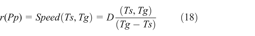
When the robot encounters an obstacle, r(Pp) will be generated to accumulate the distance and time of each step until the robot gets rid of the influence of the obstacle. A solution is selected with a lower cost.
Case retrieval
Case retrieval is always the key part in CBR technology and directly impacts the overall performance of the algorithm. Case retrieval mainly contains three processes: identify the characteristics, preliminary matches, and best selection. First of all, analyze the problem and extract relevant characteristics, identify a set of candidate cases related to the current case from the case base, and finally select one or more cases of the most relevant to the current case from the candidate case. The most commonly investigated retrieval methods by far are the k-nearest neighbors, 18 artificial neural networks, 19 knowledge-guided approaches, and inductive index approaches. 20
Because of the number of cases to be searched in our case base is small, we choose k-nearest neighbors as our retrieval method, by computing the distance between the current case and each case in the case base, the closest one will be found as the best solution.
Case retrieval is closely related with the case representation. Weighted average method is a simple similarity measure method for those case bases, which is represented by attribute-value method. The sum of all feature weightings on a case is equal to 1.
In many situations, different features have different levels of importance and contribution to the success of a case, so a reasonable weight needs to be set to reduce the searching space for the case retriever. Considering the number of feature size, we choose a method of rough estimate to assign weightings.
For a given case

The retrieval process carries through the following steps:
Step 1. Search the cases that have the same category with the present one in the case base,
Step 2. Calculate the distance between current case

Step 3. Calculate the sum of multiple distances with weighting factor of each feature, which is the total distance between current case

where formula (21) is the most common type of distance measure called Euclidean distance.
Step 4. We can get the similarity between the two cases according to the definition of given distance

When Distance = 0, SIM have a maximum value of 1, which means that the two cases are identical. When Distance = 1, SIM have a minimum value, which means that the two cases are different completely. It indicates that the larger the SIM value is, the more similar the two cases are.
Step 5. Select one or more cases whose feature is most similar to the current case, arrange those cases in a descending order according to their similarity, the similarities of all those cases are greater than a given threshold value.
For the case retriever, it is reasonable to use weights to calculate the distance between target case and each case in the same category. When it is a linear obstacle, the leftlength’s
Case adaptation
When the case retrieval is completed, we need to adapt the solution to fulfill the needs of the current case. If returned similar cases are more than one, compute the length according to the positions of the robot and the first reset goal to obtain the closest one. If necessary, modify the solution. The pseudo code of case adaptation is shown as above (Algorithm 2).
Case adaptation.

Case learning and case retaining
Case learning takes an important part in CBR system, which involves the policies and techniques of adding, deleting, and updating cases in a CBR system in order to guarantee its ongoing effectiveness and performance. In this part, case learning is measured by the cost introduced above. Cases with lower cost can play a positive role in the decision making.
If there is no similar case in the case base during case retrieval, the system will invoke MAPF to solve the current problem. The new case, its relevant solution, and r(Pp) will be retained into the case base. It not only increases the coverage of the case base but also reduces the distance between an input vector and the closest stored vector.
In addition, after case adaptation, the solution may be modified in order to adapt to the current environment.
If
Experiment
In this section, we demonstrate some simulations and actual tests to verify the efficiency and accuracy of our method. In order to facilitate our actual test, the robot is depicted as a hexagon in the simulation. First of all, the kinematical structure of the robot is described in the following subsection.
Kinematical model
The experiments are implemented using the three omni-wheel robot. The omni-wheel robot could move in any direction. Figure 4 shows the robot.

Omni-wheel robot.
Kinematical equation can be obtained from its kinematical diagram described in Figure 5.

Kinematical diagram of the omni-wheel robot.
In Figure 5,
After reasoning, Vi of each wheel can be obtained and described in the vector–matrix form as follows

where
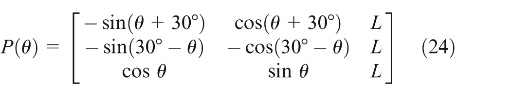
In fact, the velocity of each wheel has been given in advance. We can obtain the orientation and speed of the robot through another equation transformed by equation (25)

where

Simulation
Based on kinematical equation described above, three different obstacle cases which retrieved by the proposed two basic build-in case models have been designed to run the experiments, respectively, including one linear obstacle, one concave polygon obstacle, and one convex polygon obstacle. In order to test the performance of global planning, a complex scenario is also designed, which is composed of multi-obstacles.
To model the unknown environment in MATLAB (version: 2010a), the parameter is set as below. Size of whole map is 50 cm × 50 cm, starting point coordinate is (−20, −20), target point coordinate is (20, 20), and the velocity of the robot is 1 cm/s. There is no pause during the whole traveling process. Robot should arrive at the target point at a predetermined time; if not, the experiment result will be judged as failed. Each scenario was repeated 50 times to distinguish system with CBR from system without CBR. The distance and time below represent the average path length and average time consumption from start point to target point, respectively.
One linear obstacle
In scenario 1, the linear obstacle consists of four walls including four sides and four angles. Every side or angle is a separate case; in total, there are eight cases in this scenario. Planning path with EMMAPF method, robot will update its move direction on case base constantly by comparing dist1 with dist2 when it meets the obstacle wherever on the four sides or the four angles. At the same time, system calculates the corresponding transfer angle, and finally realizes the robot navigation and obstacle avoidance.
The specific implementation process is as follows. At first, in the first corner, the robot met an angle-type obstacle. After comparing the value between dist1 and dist2, system judged that draw toward the vertical wall will be better. It can be known that

Path with (a) “MAPF” method and (b) “EMMAPF” method in scenario 1.
As it can be seen from Table 1, “EMMAPF” method reduced the average time almost by 9.7%, and the distance from start point to target point was reduced almost by 6.2%.
Average time and distance of the path in scenario 1.

MAPF: modified artificial potential field method; EMMAPF: experience mixing with modified artificial potential field method.
One convex polygon obstacle
In scenario 2, the convex polygon consists of four walls. Every side or angle is a separate case; in total, there are eight cases in this scenario. Planning path with EMMAPF method, robot will update its move direction on case base constantly by comparing dist1 with dist2 when it met a linear obstacle in the first corner. After comparing the value between dist1 and dist2, system judged that move toward upper left will be better. It can be known that

Path with (a) “MAPF” method and (b) “EMMAPF” method in scenario 2.
As it can be seen from Table 2, “EMMAPF” method reduced the average time almost by 7.5%, and the distance from start point to target point was reduced almost by 3.0%.
Average time and distance of the path in scenario 2.

MAPF: modified artificial potential field method; EMMAPF: experience mixing with modified artificial potential field method.
One concave polygon obstacle
There are many shapes of concave obstacles. In this scenario, we chose a common shape, which shows in Figure 8 to do this simulation. The concave polygon consists of eight walls including eight sides and eight angles. Besides the identical cases, there are total nine separate cases in this scenario. In this simulation, totally there are five used cases during robot’s movement including two linear cases and three angle-type cases. The path planning result of two linear walls with border length that is equal to 14 and 2 is horizontal movement to the right. For those three-angle-type cases where the lengths of left and right side are (2, 5), (2, 7), and (14, 5), the deflective angles are

Path with (a) “MAPF” method and (b) “EMMAPF” method in scenario 3.
Scenario 3 is a concave polygon obstacle environment. Using CBR method is more effective in the performance of time and distance. The data in Table 3 show that using this method reduced the traveling time by 3.3% and distance reduced by approximately 3.2%.
Average time and distance of the path in scenario 3.

MAPF: modified artificial potential field method; EMMAPF: experience mixing with modified artificial potential field method.
Complex multi-obstacles
In scenario 4, we built an overall case base consists of triangle, trapezium, parallelogram, and the other basic obstacles which were introduced in Figure 10. Through case retrieval system, we test the most similar matching case. If there is any unreasonable path, correct it and re-store into the case base. In addition, fuzzy logic method 7 is selected to be tested in the contrast experiment. Fuzzy logic, similar to our proposed EMMAPF, is also a method to deal with path planning in unknown and dynamic environment in real time, and it could also achieve optimal local path planning.
For fuzzy logic method, the movement of the robot in the system is done by a fuzzy inference system (FIS) planner. The FIS takes four inputs. There are angle to goal (α), distance from goal (dg), distance from obstacle (d0), and turn to avoid obstacle (t0). There is a single output that measures the angle (β) that the robot should turn along the direction. The rules can be classified into two major categories. The first category of rules tries to drive the robot toward the goal. The second category of rules tries to save the robot from obstacles. If an obstacle is very near, the second category of rules becomes very dominant. A total of 11 rules are identified; these are given in Figure 9. The numbers in parentheses denote the weights.

FIS rules.
The comparison of path performance is shown in Figure 10 and Table 4.

Path with (a) “MAPF,” (b) “EMMAPF,” and (c) “Fuzzy logic” method in scenario 4.
Average time and distance of the path in scenario 4.

MAPF: modified artificial potential field method; EMMAPF: experience mixing with modified artificial potential field method.
In Figure 10, it is obvious that robot gets trapped in the local minimum problem and cannot reach the target point using fuzzy logic method, while MAPF and EMMAPF method can complete robot autonomous navigation effectively. The robot will unable to complete effective path navigation when it meets new and unknown environment, because the rules of fuzzy logic are preset. However, the actual situation is that not all the rules can be considered in advance. In this article, as described in the previous section, the local minima problem can be solved using MAPF method. Moreover, it can also be solved by our proposed EMMAPF which is an optimal method to combine MAPF with CBR mechanism. In CBR, the cases of complex obstacles can be retrieved by two basic build-in case models which is composed of “linear-type obstacle model” and “angle-type obstacle model.” In the process of the global obstacle avoidance, system will invoke CBR algorithm using its past experience to achieve obstacle avoidance when obstacles are recognized as known type; otherwise, it will invoke the “MAPF” method to solve the current problem, and the new case will be self-retained into the case base if the obstacle type is considered as an unknown. In addition, as can be seen from the data in Table 4, by comparing our proposed EMMAPF method with MAPF method, the runtime is reduced by approximately 12.1%, and the distance is reduced by 7.8%; although the time-consuming performance of fuzzy logic method is good and the path distance of local path is optimal in some cases, there exists some abnormal problems such as the path is not optimal and the target is unable to be reached when the rules of fuzzy logic are incomplete.
Simulation result analysis
Based on the experimental results, we can conclude that the path of “EMMAPF” method is more optimal than “MAPF” method and “fuzzy logic” algorithm. The path generated through “MAPF” method is safe but long and passes through many unnecessary places. Using “EMMAPF” method to obtain the available prior experience can help the robot to make the best decisions when it encounters the obstacles.
Real test
In order to control the real-time movement of the robot to verify the effectiveness of this method, we take an actual test based on a Kinect sensor with the mobile robot.
Kinect is a motion sensing input device that is used by Microsoft Xbox 360video game console and WindowsPCs. Besides the main business as a gaming device, it is also treated as a good sensor to identify the category of obstacles for robot. In brief, Kinect includes a color (RGB) camera, an infrared depth sensor, an accelerometer, four microphones, and a motor to adjust the tilt. Its detection depth is up to 5 m.
Color camera obtains an actual image of the current environment. Infrared depth sensor collects the depth data, which indicates the distance between the objects and the camera. Regardless of the light condition around the environment, Kinect could capture 640 × 480 registered image and depth points at 30 frames/s. After analyzing the related environmental information, we could obtain the features of the obstacles. Figure 11 shows the process of the experiment. We implement our experiments based on the robot operating system (ROS) platform.

The process of the experiment.
In fact, model environment depends on the sensor data type and the purpose of using generated map. Figure 12 shows how to build a model of the environment. 21

Building a model of the environment.
Mapping into two-dimensional space
In the beginning, Kinect scans the environment to generate RGB-D images. Successive frames of RGB-D information are captured during the movements of the robot at 30 frames/s, and then obtain the point clouds from the depth image. A point cloud is always defined as a set of irregular, unorganized points in three dimensions (3D). point cloud data (PCD) files contain the message including each point coordinate (x, y, and z) and the color information. Figure 13 illustrates an example of generating point cloud in our real-world test scene.
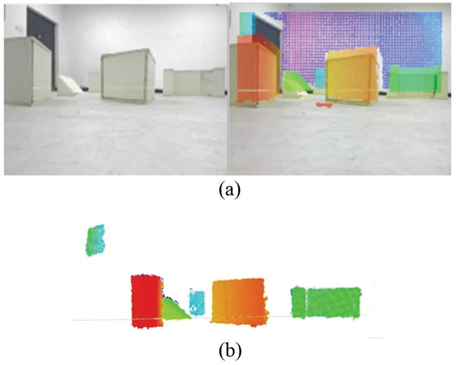
An example of generating point cloud. (a) RGB image (left) and depth information (right) taken by a RGB-D camera and (b) point cloud.
Because of the point cloud data are based on Kinect-centered coordinate, so we need to transform the points into world coordinates when we map the point cloud into a two-dimensional (2D) continuous space. Two steps have been taken. First, keep the points between the min and max height which Kinect could detect by equation (27). Second, map those point clouds into equivalent 2D continuous space by equation (28).

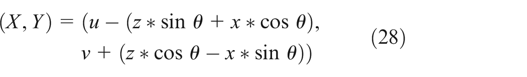
where
Figure 14 shows the effect of mapping point cloud in Figure 13 (b) into 2D space.

Map point cloud into 2D space.
The more the frames are captured, the more points are included in the 2D-mapped space. The 2D-mapped points with new frames would be added into the world coordinate with the increase in time.
Data clustering
The next step is to cluster the points of 2D map; some kinds of clustering algorithm have been tried to apply in data clustering; in this research, density-based spatial clustering of applications with noise (DBSCAN) is the best approach which is capable of finding arbitrarily shaped clusters. It is very flexible with unusual shape of dense point areas. Figure 15 illustrates the resulting clusters which could represent one shape in the space.

Data clustering by DBSCAN algorithm.
Concave-hull approach
P Wasmeier 22 implemented a function in MATLAB called hullfit, which could calculate a concave-hull of a data set. Two parts are included in this algorithm.
First, apply the concave-hull to obtain vertices of corresponding convex-hull and classify them as clockwise. Next, calculate the distances among each two neighbors’ vertices to find any distance greater than maximum allowed distance. If any points returned, use some conditions to find another proper point in the data set as the next vertex.
More detailed description is introduced in Mojtahedzadeh. 23 Here, we apply the function hullfit to represent obstacles with the best polygons to fit. Figure 16 shows one final model of the environment during the robot moving to the target.

The final model of the environment.
Thus, we could get the category of the obstacle’s front shape by the Kinect sensor, such as line or concave polygon, which is the useful information of the obstacles used to complete the path planning. We imitate scenario 4 to verify the efficiency of “EMMAPF” algorithm in real world. The size of the area is 5 m × 5 m. Kinect is placed in the front of the omni-wheel robot.
The black dot in the top right corner of the scene is the target. We set the origin velocity of the robot at 0.1 m/s. Figure 17 shows the actual process of robot navigation in a complex multi-obstacle environment. The information of the obstacles is unknown in advance.

Process of the robot using “EMMAPF” method in a complex multi-obstacle environment.
Table 5 illustrates the statistical data of experiments in simulation and actual test. Time used in actual test is a little more than in simulation, while distance is shorter. This deviation is caused by the fiction that exists between the wheels of robot and the floor.
Comparison between simulation and actual test.

As it can be seen from Figure 18, two paths are shown in different colors. Blue line represents the path in simulation environment, while the red line represents the actual path in real-time physical test environment. Except for the robot traveling around the corner, the deviation of the path is small. Figure 19 records that the path deviation exists on each moment in the movement. In fact, the deviation is small (<0.1 m) and is acceptable. So, we can conclude that the “EMMAPF” algorithm could be applied in the real world successfully.
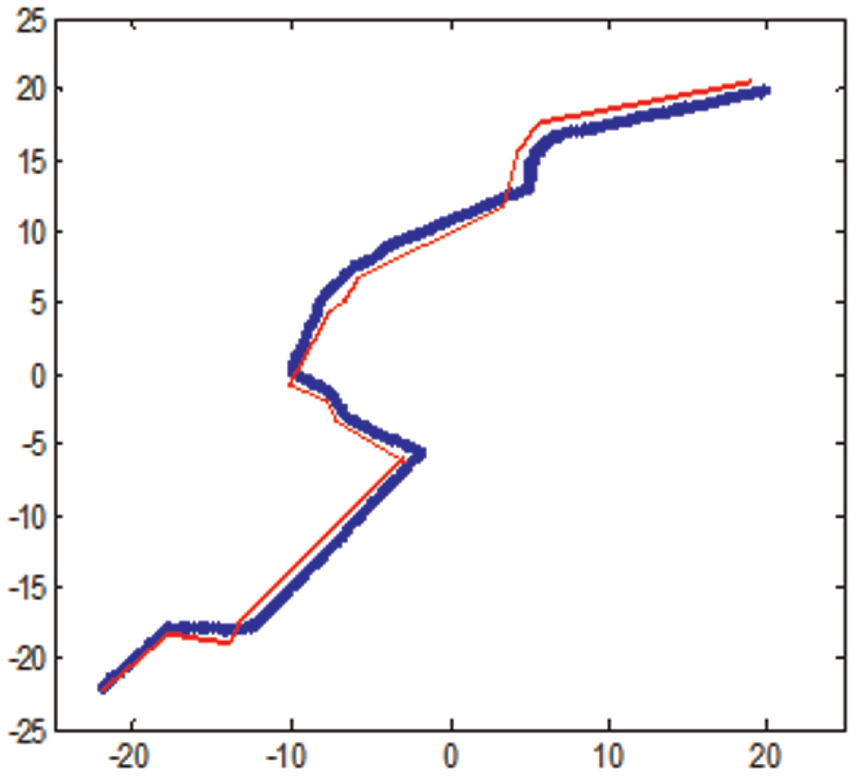
A planned path by simulation (blue line) and an actually followed path (red line) using “EMMAPF” method.

Deviation between the planned path and the actually followed path.
Conclusion and future work
In this article, a new approach EMMAPF which combines case-base reasoning method with the modified APF method is put forth to get an optimal path and better algorithm efficiency. In CBR, we innovatively consider that all the complex obstacles are retrieved by two kinds of basic build-in obstacle models (linear obstacle and angle-type obstacle). In the process of the global obstacle avoidance, system will invoke CBR algorithm using its past experience to achieve obstacle avoidance when obstacles are recognized as known type; otherwise, it will invoke the “MAPF” method to solve the current problem, and the new case will be retained into the case base if the obstacle type is considered as an unknown. In simulations, three different obstacle cases which retrieved by the proposed two basic build-in case models have been designed to run the experiments, respectively, including one linear obstacle, one concave polygon obstacle, and one convex polygon obstacle. In order to test the performance of global planning, a complex scenario is also designed, which is composed of multi-obstacles. We illustrated the obstacle avoidance process and effect of those four obstacle cases using our proposed EMMAPF compared with MAPF and fuzzy logic algorithm. In actual test, by acquiring the RGB-D images from the Kinect sensor and building the model of the final environment, robot could obtain the useful information of the obstacles and utilize the “EMMAPF” method to deal with path planning in unknown and dynamic environment in real time. According to simulation and actual test, we can come to the conclusion that this method has been proved applicable to the dynamic real-time obstacle avoidance under unknown and unstructured environment, and it greatly improved the performance of robot path planning that not only reduced the time consumption but also shorten the moving distance.
In future, there are two major issues that we need to pay more attention. One is to improve the performance of CBR in real time, some measures need be taken to shorten the time in searching and matching; otherwise, time delay in CBR mechanism would lead to the failure of the obstacle avoidance. The other issue is to improve the accuracy of building a model of the environment. More different methods should be studied and compared in data clustering. The detection of the obstacles in the environment has a significant effect on the results of the “EMMAPF” method. With the development of this method, our system will become a true real-time system to deal with path planning for mobile robot in the future.
Footnotes
Acknowledgements
This article is a revised and expanded version of a paper entitled “Experience Mixed the Modified Artificial Potential Field Method” which presented at the IEEE/RSJ International Conference on Intelligent Robots and Systems (IROS 2013), held at Tokyo, Japan, during 3–8 November 2013.
Academic Editor: Long Cheng
Declaration of conflicting interests
The author(s) declared no potential conflicts of interest with respect to the research, authorship, and/or publication of this article.
Funding
The author(s) disclosed receipt of the following financial support for the research, authorship, and/or publication of this article: This work was supported by the National Natural Science Foundation of China (Grant No. 61175094).