Predicting fatigue crack growth under variable amplitude loadings with usage monitoring data

Abstract

For complex engineering systems, there is an increasing interest in the use of structural health monitoring systems to estimate the current state of damage (diagnosis) and to predict the behavior of the damage in the future (prognosis). For fatigue crack growth, one challenge in prognosis is to predict dynamic stress history at the location of damage. In this article, a method of predicting fatigue crack growth in aircraft panels is proposed under variable amplitude loading. A simple analytical–numerical method is proposed to calculate dynamic stress history from the usage monitoring data. A variable amplitude fatigue analysis is then conducted through the use of a fatigue crack growth model with the extended finite element method. Numerical examples show that the effect of underload and overload is significant in fatigue crack growth. It is also indicated that the crack growth rate and direction can significantly change under the multi-axial loading environment.

Introduction

The current aircraft maintenance procedures are schedule-based. After a number of flights, an aircraft is taken to a hangar where it is inspected for damage. If damage is identified, it is repaired and the aircraft continues to operate until the next scheduled maintenance. Structural health monitoring aims to reduce the number of inspections needed during the lifecycle of an aircraft through the addition of sensors. The data from these sensors can be used to estimate the size and location of damage within a panel. Furthermore, the evolution of the size and location of the damage can be used to identify the damage growth behavior of the panel, and accordingly, the remaining useful life can be estimated. These techniques are still in development and are not sufficiently developed for wide-spread use.

The estimation of the damage growth behavior and/or remaining life is often referred to as prognosis. Prognosis models for fatigue crack growth work under the assumption that a stress history is available, which is often not the case. It has been proposed to add strain gauges at specific locations in a panel in order to estimate stress near the crack location. However, for the case of aircraft, the location of the crack is not given a priori, and the addition of sensors will increase the weight of the structure, which is always a concern. In this article, a method is introduced to use readily available service data from an aircraft such as accelerations and angle of attack for the estimation of stress history at a location on an aircraft wing box. The stress history can then be used in a prognosis model in conjunction with structural health monitoring data.

In this article, the stress history identified from the service data is used for a bi-axial, variable amplitude fatigue crack growth analysis. Due to the non-proportional bi-axial load history, traditional methods that group multiple loading cycles into a single finite element simulation are not applicable, as each cycle has a unique preferred direction of crack growth. To this end, a multi-axial rain-flow counting method is proposed that can also preserve the order of load cycles. A modified version of the Paris model ¹ which considers the effects of variable amplitude loading is used to determine the magnitude of crack growth at each iteration according to the mixed-mode stress intensity factors identified by an extended finite element method (XFEM)^2–4 analysis. The results of XFEM analysis are then used in the critical plane approach ⁵ to determine the preferential crack growth direction, which is cycle-dependent for non-proportional loading. In order to reduce the cost associated with the repeated simulations, the XFEM stiffness matrix is factored and directly modified to account for the small changes to the stiffness matrix that occur as a result of crack growth. ⁶

The article is organized as follows: in section “Summary of usage monitoring data,” the usage monitoring data that are used in calculating stress history are summarized. A hybrid analytical and numerical approach is presented to calculate dynamic stress history using the usage monitoring data and finite element analysis in section “Conversion of usage monitoring data to stress history.” The multi-axial, variable amplitude crack growth model is presented in section “Crack growth model” with multi-axial rain-flow counting. In section “XFEM,” the XFEM is used in modeling crack growth. The numerical results are presented in section “Numerical results,” followed by conclusions and discussions in section “Conclusion and future work.”

Summary of usage monitoring data

Usage monitoring data from an aircraft were provided by the Air Force Research Laboratory. ⁷ The data provided were normalized and no particular aircraft which corresponded to the data was given. Therefore, the results presented here cannot represent a specific airplane; rather, it should be understood as the generic behavior of airplanes. The data were separated into 19 independent flights, each of which contained normalized data for the following parameters: 6 accelerations (normal, lateral, longitudinal, roll, pitch, and yaw), 3 angular speeds (roll, pitch, and yaw), airspeed, altitude, angle of attack, flap angle, fuel quantity, and Mach number. The total number of data points for the all 19 flights was 180,588. In this article, only the following data were used in the prediction of a stress history: normal acceleration, roll acceleration, airspeed, angle of attack, fuel quantity, and Mach number. The usage monitoring data were recorded at certain events (e.g. landing gear up/down) or at the maxima or minima of an acceleration component. It was assumed that the effect of the roll acceleration would result in changes in the banking angle of the airplane. This effect was considered by scaling the roll acceleration to the banking angle and using the banking angle to predict the stresses upon the airplane wing.

As the usage monitoring data were normalized, it was necessary to scale the data according to what could be expected for a particular airplane. It was chosen to consider a panel located along the wing box of an airplane. The normalized data were scaled linearly between the maximum and minimum values for a given parameter x according to the following relationship

$$x_i^{\mathrm{scaled}}=x_{min}^{\mathrm{scaled}}+\frac{(x_i^{\mathrm{norm}}-x_{min}^{\mathrm{norm}})(x_{max}^{\mathrm{scaled}}-x_{min}^{\mathrm{scaled}})}{x_{max}^{\mathrm{norm}}-x_{min}^{\mathrm{norm}}}$$

(1)

where the maximum and minimum scaled values for x are $x_{max}^{\mathrm{scaled}}$ and $x_{min}^{\mathrm{scaled}}$ , respectively; the maximum and minimum normalized values are $x_{max}^{\mathrm{norm}}$ and $x_{min}^{\mathrm{norm}}$ , respectively; the scaled data point is $x_i^{\mathrm{scaled}}$ ; and the normalized data point is $x_i^{\mathrm{norm}}$ . The values for $x_{max}^{\mathrm{scaled}}$ and $x_{min}^{\mathrm{scaled}}$ for each of the parameters used in the stress analysis are given in Table 1. The values of $x_i^{\mathrm{norm}}$ , $x_{max}^{\mathrm{norm}}$ , and $x_{min}^{\mathrm{norm}}$ are flight dependent and obtained from individual flight data.

Table 1.

Ranges for parameters used in the conversion of the normalized data to scaled data.

Parameter	Variable	Unit	Maximum	Minimum	Reference
Normal acceleration	anorm	g	1.5	0.75
Roll acceleration	θB	°	30	0
Airspeed	V	m/s	851	0	Boeing 8
Angle of attack	A	°	10	0
Fuel quantity	mfuel	kg	50,000	800	Boeing 8 and Wikipedia 9
Mach number	M	N/A	0	0.80	Boeing 8

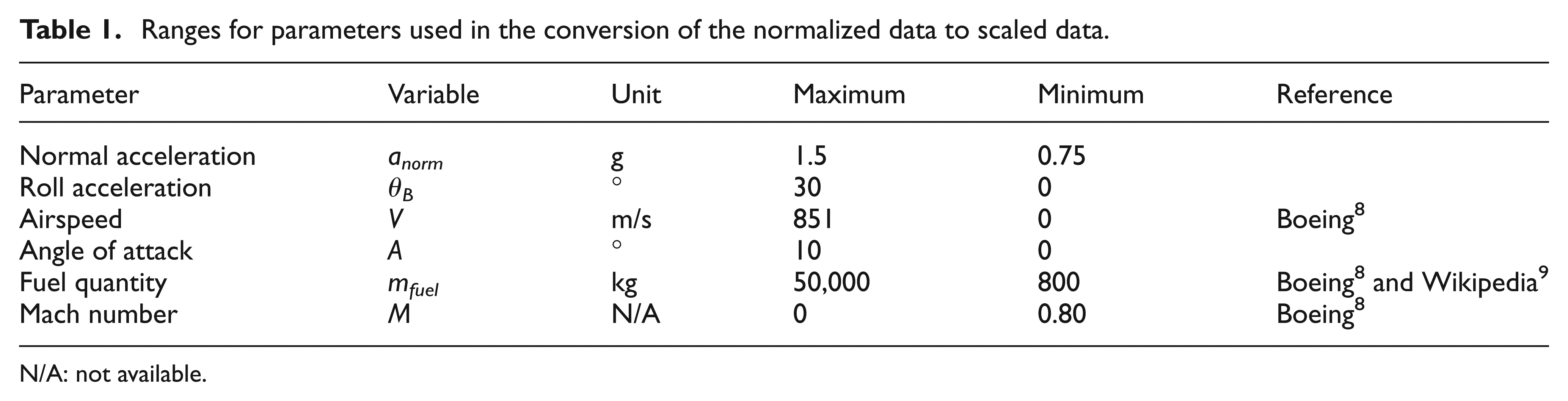
N/A: not available.

Conversion of usage monitoring data to stress history

The usage monitoring data for the airplane need to be converted into a stress history, allowing the stress to be approximated at any location on the airplane wing through the use of a finite element model of the wing box as shown in Figure 1. A commercial finite element analysis program, ABAQUS, is used. Although a high-fidelity fluid–structure interaction analysis is required to calculate the dynamic stress history of the wing box, it will be computationally too expensive to follow a complete history of usage data. In addition, such a high-fidelity simulation may not be necessary because the objective is to estimate main trends of stress amplitude variation. In this article, a simple method of estimating the stress history is presented using static finite element analyses and the analytical model of load distribution.

Figure 1.

Example of a wing box with span s and chord length c.

Three linear elastic analyses were performed on the finite element model for a pressure distribution P(x, y) with a maximum value of 1 corresponding to lift acting upon the wing. Each of the three analyses corresponded to a different angle of attack (α = 0°, 5°, and 10°) and, thus, a different P(x, y). To approximate the lift distribution, 80% of P(x, y) was applied to the top surface of the wing box while 20% of P(x, y) was applied to the bottom of the wing box. A fourth analysis was performed which considered the effect of a uniform drag pressure distribution which acted upon the leading and trailing edge of the wing box, again with a maximum value of 1. To approximate the drag distribution, 80% of the uniform pressure distribution was applied to the leading edge of the wing and 20% was applied to the trailing edge.

The pressure distribution P(x, y) is assumed to follow the form

$$P(x,y)=w_o{p}_u(u)p_w(w)$$

(2)

where w_o is the magnitude of P(x, y) at the maximum location, p_u(u) is the normalized chord-wise pressure distribution with u = x/c being the normalized coordinate in x-direction, and p_w(w) is the normalized span-wise pressure distribution with w = y/s being the normalized coordinate in y-direction. Both p_u(u) and p_w(w) are normalized, such that their maximum magnitudes are one. The chord-wise pressure distribution was represented as a sixth-order polynomial as

$$p_u(u)=a_6{u}^6+a_5{u}^5+a_4{u}^4+a_3{u}^3+a_2{u}^2+a_{1}u+a_0$$

(3)

where the location of maximum pressure is a function of the angle of attack. Unique coefficients in equation (3) were calculated for each angle of attack. The span-wise pressure distribution was chosen to follow

$$p_w(w)=\sqrt{1-w^2}$$

(4)

from the work of Choklovshi, ¹⁰ Lobert, ¹¹ and Pippy. ¹² The normalized chord-wise and span-wise pressure distributions are shown in Figure 2. From the finite element analyses within ABAQUS, the bi-axial stress components for a location on the top of the wing (−4.32, 7.42) m of the wing box were calculated and are summarized in Table 2.

Figure 2.

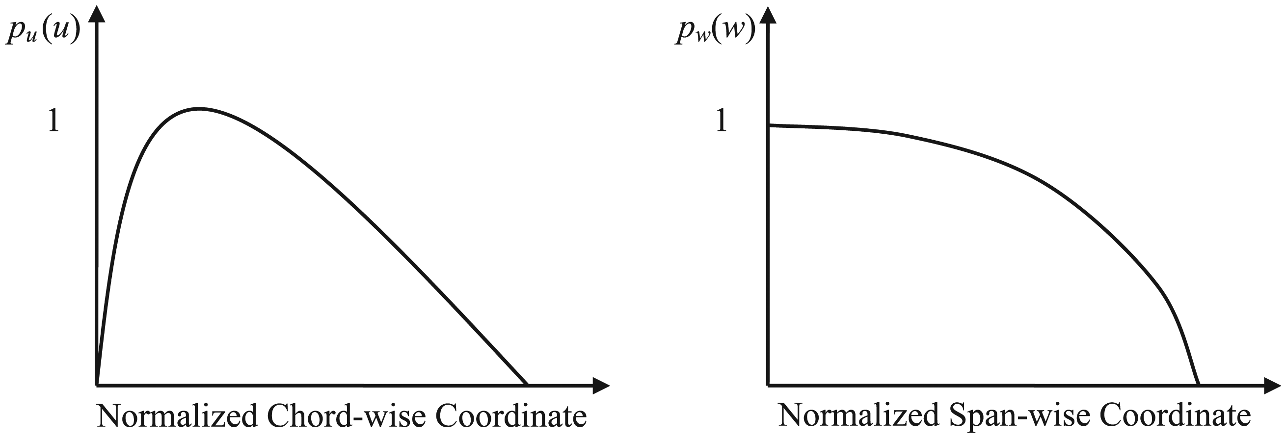
Normalized chord-wise and span-wise pressure distributions p_u(u) and p_w(w).

Table 2.

Bi-axial stress components for each wing box analysis for unit pressure distribution.

Analysis	σxx (MPa)	σyy (MPa)	σxy (MPa)
Drag	22.3	−33.4	32.2
Lift, α = 0°	134	483	298
Lift, α = 5°	133	484	296
Lift, α = 10°	131	480	291

In order to consider the intermediate values for the angle of attack between 0° and 10°, a kriging^13–16 surrogate model was fit to the stress values in Table 2 and used to evaluate the stress component from lift ${\sigma }_{\mathrm{ij}}^L$ for any angle of attack. This is similar to interpolating the lift stress using the stress values at three angles of attack. Since the variation in stress with respect to the angle of attack is not significant, the error in the surrogate model can be negligible. Using the surrogate model, the stress at a point is

$${\sigma }_{\mathrm{ij}}=w_o{\sigma }_{\mathrm{ij}}^L(\alpha )+q_o{\sigma }_{\mathrm{ij}}^D$$

(5)

where w_o is the maximum value of lift pressure distribution, q_o is the maximum value of drag pressure distribution, and ${\sigma }_{\mathrm{ij}}^L$ and ${\sigma }_{\mathrm{ij}}^D$ are, respectively, the stress components corresponding to lift and drag pressure distributions with unit magnitude. The values of ${\sigma }_{\mathrm{ij}}^D$ and ${\sigma }_{\mathrm{ij}}^L$ are given in Table 2. The stress components in Table 2 and equation (5) can be thought of as stress influence coefficients, corresponding to w_o = 1 for the lift and q₀ = 1 for the drag. Therefore, the stress history can be obtained if w_o, q₀, and α can be calculated from the usage monitoring data.

From the analytical model in Pippy, ¹² the maximum values of lift and drag pressure distributions are given as

$$w_o=\frac{C_L(m_{\mathrm{empty}}+m_{\mathrm{fuel}})a_{\mathrm{norm}}}{V_L\cos {\theta }_B}$$

(6)

where C_L is the lift coefficient, m_empty is the empty weight of the aircraft (86,070 kg ⁸ ), V_L is the volume under the P(x, y) surface, and ${\theta }_B$ is the bank angle and

$$q_o=\frac{a_{\mathrm{norm}}{C}_D(m_{\mathrm{empty}}+m_{\mathrm{fuel}})\tan {\theta }_B}{{\theta }_B{C}_L{V}_D}$$

(7)

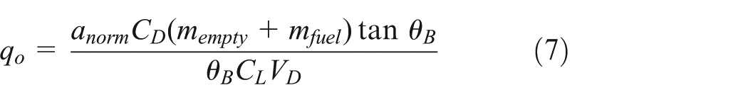
where C_D is the drag coefficient and V_D is the volume under the drag pressure distribution. The lift coefficient C_L is related to the angle of attack ¹⁷ as

$$C_L=0.11\alpha +0.4$$

(8)

and the drag coefficient C_D is related to the Mach number ¹⁸ as

$$C_D=\frac{M}{4}+0.13$$

(9)

For the given time history of normal acceleration, roll acceleration, airspeed, angle of attack, fuel quantity, and Mach number, the time histories of w₀ and q₀ are calculated, from which the histories of stress components are calculated from equation (4). A sample of the calculated stress history for all 19 flights and the corresponding 180,588 data points for each bi-axial stress component is given in Figure 3.

Figure 3.

Bi-axial stress history for a subset of the 180,588 data points corresponding to the 19 flights.

Crack growth model

In this article, fatigue crack growth is predicted using a fatigue crack growth model which is governed by an ordinary differential equation. ¹⁹ The fatigue crack growth model uses the stress intensity factor range for a particular cycle as the driving force for fatigue crack growth. Recall, the normalized flight data were previously converted into a bi-axial stress history. However, this stress history is not given in terms of cycles, but rather is simply a series of data points.

The classical way to convert a stress time history into a cyclic stress history for use in a fatigue crack growth model is through the use of the rain-flow counting algorithm.^20–22 In this algorithm, the number of cycles that have the same stress range is counted together and contributed to the damage using a fatigue model. However, this approach is not directly applicable to this analysis because there are three stress components to the bi-axial loading. Performing rain-flow counting on each of the components would result in different cyclic stress histories. It is likely that the number of cycles as well as the data points in the history data corresponding to peaks and valleys for the cycles would not agree, which is necessary if finite element simulations are used to find ΔK for each cycle.

Therefore, the bi-axial stress histories are converted into an equivalent stress history (e.g. Von Mises stress ²³ ). The rain-flow counting is then performed upon this equivalent stress. The cycles were ordered by increasing data point numbers corresponding to the beginning of a cycle. This helps to retain the ordering of the applied stresses, which is necessary for the load interactions to be properly considered. Finally, the cycles identified by the rain-flow analysis are mapped back onto the individual stress components. This enables each cycle to be modeled with a finite element simulation and the cyclic bi-axial stresses to share locations of maxima and minima. This algorithm is outlined in Figure 4. In this article, the rain-flow counting algorithm of Nieslony ²⁴ is used, which follows ASTM E 1049, Standard Practices for Cycle Counting in Fatigue Analysis. The conversion from stress history into cyclic stress history reduces the data from 180,588 points to 37,007 cycles as shown in Figure 5. As with the stress data, the cyclic stress history is non-proportional, bi-axial, and has variable amplitudes in nature.

Figure 4.

Conversion of bi-axial data into cyclic data for use in a fatigue crack growth model.

Figure 5.

Cyclic stress history identified for a subset of all stresses through rain-flow counting of an equivalent stress model.

When modeling crack growth under variable amplitude loading, the critical phenomena to capture are the interactions between the loading cycles and the effects of the stress ratio R. The stress ratio R is the ratio of the minimum to maximum stress during a particular loading cycle. A maximum in the loading history increases the crack tip plasticity, which retards future crack growth, while a minimum in the loading history decreases the crack tip plasticity, which accelerates future crack growth. One strategy for capturing this behavior is to explicitly model the plasticity using either traditional ²⁵ or XFEMs.^26,27 However, for fatigue crack growth, plasticity is highly localized around the crack tip and it has been shown^25–27 that the stress intensity factors are not significantly different under the confined plasticity assumption. Therefore, the choice here was to model the plasticity through the use of a modified Paris model ¹ which considers the effects of the crack tip plasticity on the crack growth rate by including additional material constants. This helps to further improve the computational efficiency of fatigue crack growth analysis for a non-proportional variable amplitude case where each cycle must be modeled explicitly. The modified version of the Paris model used here is given as

$$\frac{\mathrm{d}a}{\mathrm{d}N}=C[{(M_R{M}_P\Delta K)}^m-\Delta K_{\mathrm{th}}^m]$$

(10)

where C is the modified Paris model constant for R = 0, m is the modified Paris model exponent for R = 0, M_R is a corrector for non-zero R values, M_P is a corrector for the plasticity effect created by load interactions, ΔK is the stress intensity factor range, and ΔK_th is the threshold stress intensity factor range, under which the crack would not grow.

In equation (10), the parameter M_R is defined as

$$M_R=\{\begin{array}{c}\hfill {(1-R)}^{-{\beta }_1}-5\le R<0\hfill \\ \multicolumn{1}{c}{{(1-R)}^{-\beta }0\le R<0.5}\\ \multicolumn{1}{c}{{(1.05-1.4R+0.6R)}^{-\beta }0.5\le R<1}\end{array}$$

(11)

where two additional material constants β and β₁ are introduced and used to compensate for non-zero R values to R = 0. This allows for a single value to be used for C and m regardless of R, which is not the case with many models. The parameter M_P in equation (10) considers the effect of the evolution of the plastic zone at the crack tip as

$$M_P=\{\begin{array}{c}\hfill {\left(\frac{r_y}{a_{\mathrm{OL}}+r_{\mathrm{OL}}-a_i-r_{\Delta }}\right)}^n{a}_i+r_y<a_{\mathrm{OL}}+r_{\mathrm{OL}}-r_{\Delta }\hfill \\ \multicolumn{1}{c}{1a_i+r_y\ge a_{\mathrm{OL}}+r_{\mathrm{OL}}-r_{\Delta }}\end{array}$$

(12)

where n is an exponent used to accelerate or retard crack growth due to load interactions, r_y is the plastic zone radius for the current crack geometry, r_OL is the plastic zone size for the crack when the overload occurred, and r_Δ is the reduction in r_OL due to an underload. Further details on the necessary experiments to determine β₁, β, and n are available. ¹ The plastic zone radii are

$$\begin{array}{l}{r}_y={\alpha }_p{\left(\frac{K_I^{\max }}{{\sigma }_y^{+}}\right)}^2;\mathrm{\hspace{1em}}{r}_{OL}={\alpha }_p\left(\frac{K_I^{OL}}{{\sigma }_y^{+}}\right);\\ r_{\Delta }={\alpha }_p{\left(\frac{K_{I,i-1}^{\min }-K_{I,i}^{\min }}{{\sigma }_y^{-}}\right)}^2\end{array}$$

(13)

where α_p is a plastic zone correction factor, $K_I^{max}$ is the maximum Mode I stress intensity factor for the current cycle, $K_{I,i-1}^{min}$ is the minimum Mode I stress intensity factor for the previous cycle, $K_{I,i}^{min}$ is the minimum Mode I stress intensity factor for the current cycle, $K_I^{\mathrm{OL}}$ is the Mode I stress intensity factor when the overload occurred, ${\sigma }_y^{+}$ is the tensile yield stress, and ${\sigma }_y^{-}$ is the compressive yield stress. This model has been validated against sets of experimental data of variable amplitude fatigue loadings. ¹

While the modified Paris model in equation (10) gives the magnitude of the fatigue crack growth at a particular cycle, it does not specify the direction. While there are many options available for predicting the direction of crack growth,^28–31 the critical plane approach ⁵ is used here. The critical plane approach was developed based on the observation that fatigue crack growth in many metallic materials did not follow the direction predicted by maximum tensile stress. Additional material properties are used which result in the determination of the crack growth direction along some critical plane for a given material. The main advantage of the critical plane approach compared to a simpler model, such as the maximum circumferential stress criterion, is that an added emphasis is placed upon shear-dominated failure while a model such as the maximum circumferential stress criterion emphasizes tensile-dominated failure. The direction of crack growth predicted by the critical plane approach in the crack tip coordinate system is

$$\theta =\varphi +\gamma$$

(14)

where ϕ is given by

$$\varphi =\frac{1}{2}\arctan \left(\frac{2K_{\mathrm{II}}}{K_I}\right)$$

(15)

Here, K_I and K_II are the Mode I and II stress intensity factors, respectively, and γ follows the relationship

$$\gamma =\{\begin{array}{c}\hfill \frac{1}{2}\arccos \left[\frac{-2+\sqrt{4-4(1/s^2-3)(5-1/s^2-4s^2)}}{2(5-1/s^2-4s^2)}\right]s\le 1\hfill \\ \multicolumn{1}{c}{0s>1}\end{array}$$

(16)

where the value of s is given as

$$s=\frac{K_{\mathrm{II},\mathrm{d}a/\mathrm{d}N}}{K_{I,\mathrm{d}a/\mathrm{d}N}}$$

(17)

where K_I,_da/dN and K_II,_da/dN are the Mode I and II stress intensity factors corresponding to a particular crack growth rate da/dN. The mixed-mode stress intensity factors K_I and K_II are converted into an equivalent stress intensity factor range ΔK according to the work of Liu and Mahadevan. ⁵

XFEM

The classical finite element method requires the finite element mesh to conform to the domain of interest. ³² In terms of modeling numerous crack growth iterations, the domain of interest is constantly changing due to crack growth. The need to recreate the mesh, even locally around the crack tip, is a challenge and leads to increased computational cost. The XFEM^2–4 exploits the partition of unity finite element method to include additional functions, often referred to as enrichment functions, into the displacement approximation. Enrichment functions allow for the discontinuity in the domain introduced by a crack to be modeled without the need to create the finite element mesh as the discontinuous geometry evolves with time. The displacement approximation associated with the XFEM becomes

$${\mathbf{u}}^h(\mathbf{x})=\sum _{\mathrm{I}}{\mathrm{N}}_{\mathrm{I}}({\mathbf{u}}_{\mathrm{I}}+\mathrm{H}{\mathbf{a}}_{\mathrm{I}}+\sum _{\mathrm{J}=1}^4{\Phi }_{\mathrm{I},\mathrm{J}}{\mathbf{b}}_{\mathrm{I},\mathrm{J}})$$

(18)

where N_I are the traditional finite element shape functions, u_I are the traditional nodal degrees of freedom (DOFs), H is the Heaviside enrichment function, a_I are additional DOFs associated with the Heaviside enrichment function, Φ_I,J are the crack tip enrichment functions, and b_I,J are the additional DOFs associated with the crack tip enrichment functions. It should be noted that the enrichment functions take values of 0 throughout much of the domain and the additional DOFs are located only locally around the discontinuity as shown in Figure 6, where circles denote nodes enriched with the Heaviside function and squares denote nodes enriched with the crack tip enrichment function; filled circles and squares denote new enriched nodes for the current iteration while open circles and squares denote previously enriched nodes.

Figure 6.

XFEM mesh with enriched nodes: (a) initial geometry and (b) after crack growth iteration.

The traditional Galerkin method may be applied to the displacement approximation given by equation (18) to yield a system of equations of the form

$$\left[\begin{array}{ccc}\hfill {\mathbf{K}}_{\mathrm{uu}}\hfill & \hfill {\mathbf{K}}_{\mathrm{au}}^{\mathrm{T}}\hfill & \hfill {\mathbf{K}}_{\mathrm{bu}}^{\mathrm{T}}\hfill \\ \multicolumn{1}{c}{{\mathbf{K}}_{\mathrm{au}}}& \hfill {\mathbf{K}}_{\mathrm{aa}}\hfill & \hfill {\mathbf{K}}_{\mathrm{ba}}^{\mathrm{T}}\hfill \\ \multicolumn{1}{c}{{\mathbf{K}}_{\mathrm{bu}}}& \hfill {\mathbf{K}}_{\mathrm{ba}}\hfill & \hfill {\mathbf{K}}_{\mathrm{bb}}\hfill \end{array}\right]\left\{\begin{array}{c}\hfill \mathbf{u}\hfill \\ \multicolumn{1}{c}{\mathbf{a}}\\ \multicolumn{1}{c}{\mathbf{b}}\end{array}\right\}=\left\{\begin{array}{c}\hfill {\mathbf{f}}_{\mathrm{u}}\hfill \\ \multicolumn{1}{c}{{\mathbf{f}}_{\mathrm{a}}}\\ \multicolumn{1}{c}{{\mathbf{f}}_{\mathrm{b}}}\end{array}\right\}$$

(19)

where ${\mathbf{K}}_{\mathrm{uu}}$ are the traditional finite element stiffness components; ${\mathbf{K}}_{\mathrm{aa}}$ are the Heaviside stiffness components; ${\mathbf{K}}_{\mathrm{bb}}$ are the crack tip stiffness components; and ${\mathbf{K}}_{\mathrm{au}}$ , ${\mathbf{K}}_{\mathrm{bu}}$ , and ${\mathbf{K}}_{\mathrm{ba}}$ are the stiffness components coupling the traditional, Heaviside, and crack tip displacement terms, respectively. In the conventional finite element method or XFEM, the stiffness matrix needs to be generated at each crack growth iteration, and the system of equations is solved for nodal DOF (u, a, and b). This requires a tremendous amount of computational resources as the fatigue crack growth often comes with millions of loading cycles. It should be noted from Figure 6 that only a small portion of the total stiffness matrix contains enriched terms; in practice, it is common for the enriched number of enriched DOFs to be between 1% and 5% of the total number of DOFs in the system of equations.

As crack growth occurs, only a small portion of the global stiffness matrix may be modified; new additions are made to the Heaviside components ${\mathbf{K}}_{\mathrm{aa}}$ and ${\mathbf{K}}_{\mathrm{au}}$ and all crack tip components ${\mathbf{K}}_{\mathrm{bb}}$ , ${\mathbf{K}}_{\mathrm{bu}}$ , and ${\mathbf{K}}_{\mathrm{ba}}$ will change as a result of the changing crack tip position. In practice, it is possible to factor equation (19) using the Cholesky factorization algorithm. This factorization can then be modified directly to consider the effects of the changes to the enriched components of the stiffness matrix which occur due to crack growth through the use of row add and row delete operations. ⁶ Numerical experiments have shown a savings of about 80% in the assembly of the stiffness matrix and 70% in the factorization and solving of the system of linear equations through the use of this method.

Due to the non-proportionality of the bi-axial stress components, two analyses are required for each cycle which was identified by the rain-flow counting method: one at the maximum and other at the minimum of each cycle. This results in the need for twice the number of simulations as there are loading cycles, or 74,014 XFEM analysis. In practice, the authors’ MATLAB XFEM code ³³ was coupled with CHOLMOD ³⁴ through the use of a MEX file to enable efficient computation of the 74,014 repeated simulations. In order to ensure efficiency of the updating algorithm, a fill-reducing ordering is calculated using the approximate minimum degree ordering algorithm ³⁵ for a matrix which contains all possible connectivities including traditional, Heaviside, and crack tip components. Without this algorithm, it would be challenging to consider the cycle-by-cycle load history for the non-proportional bi-axial variable amplitude loading history, which was identified from the usage monitoring data.

Numerical results

The material properties used in the numerical results were chosen to represent aluminum 7075-T6 as follows: Young’s modulus of 70 GPa, Poisson’s ratio of 0.3, yield stress of 520 MPa, threshold stress intensity factor range of 2.2 MPa, modified Paris model constant of 6.85E−11, modified Paris model exponent of 3.21, negative R-ratio correction β₁ of 0.84, positive R-ratio correction β of 0.70, and plasticity acceleration/retardation exponent n of 0.3. ¹

First, the effect which an overload or underload has upon fatigue crack growth according to the modified Paris model ¹ is studied. A simple block loading spectrum is used to illustrate the idea where the block loading is shown in Figure 7. Four cases are considered: no overload or underload, an overload with no underload, an underload with no overload, and an overload and an underload. Recall, that the general effect of an overload is an increase in plasticity which will retard future crack growth. Inversely, an underload will accelerate future crack growth. For this example problem, the values for the stress in the block loading spectrum were defined as σ₁ = 50 MPa, σ₂ = 150 MPa, σ₃ = 250 MPa, and σ₄ = 350 MPa. The stress intensity factor was predicted for the center crack in an infinite plate model with stress range Δσ and half crack length a as

$$\Delta K=\Delta \sigma \sqrt{\pi a}$$

(20)

Figure 7.

Block loading spectrum used to examine effects of overload and underload upon crack growth curve.

Crack growth stopped once the characteristic crack length reached 50 mm from an initial crack size of 5 mm.

The results of this simple variable amplitude fatigue analysis are presented in Figure 8. It can be noted that, as expected, the presence of an overload decreases the crack growth rate (e.g. increasing number of cycles to reach a particular crack length) when compared to the constant amplitude case. For an underload, the increased crack growth rate occurs due to the reduction in crack tip plasticity. The combination of an overload and an underload results in a crack growth rate that is slower than the constant amplitude case, but faster than the overload-only case. The differences between these cases represent the need to consider the crack tip plasticity when predicting fatigue crack growth under variable amplitude loading.

Figure 8.

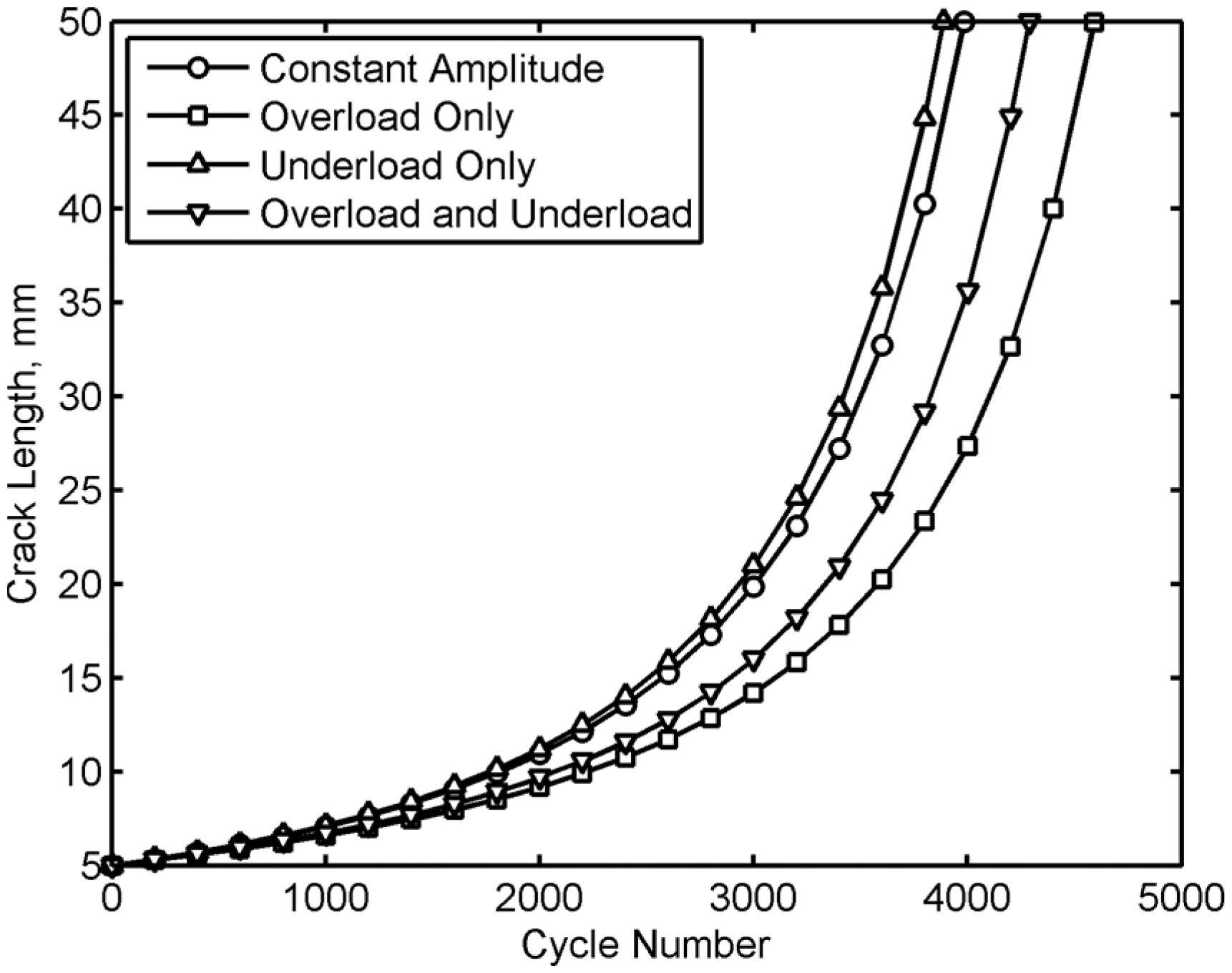
Comparisons of the crack growth rate for constant amplitude and variable amplitude loading under a block loading spectrum.

The example problem to which the non-proportional bi-axial stress cycles identified from the usage monitoring data were applied was that of a square plate with sides of length of 0.1 m containing an edge crack of 5 mm as shown in Figure 9. The 37,007 bi-axial stress cycles were modeled as 74,014 XFEM simulations. The magnitude of crack growth was predicted using the modified Paris model, and the direction of crack growth was predicted using a critical plane approach.

Figure 9.

Simplified plate geometry used for the fatigue analysis from service data.

A structured XFEM mesh was used where the average element size was 1/200 m. After performing an analysis for several hundred cycles, it was noted that the cyclic stresses did not create sufficiently large stress intensity factor ranges to exceed the threshold stress intensity range. To encourage crack growth to occur, all stresses were magnified by a factor of 10, which created periodic crack growth. This resulted in crack growth occurring in about 2500 of the 37,007 cycles. The resulting crack growth as a function of cycle number is given in Figure 10 and the predicted growth path is shown in Figure 12.

Figure 10.

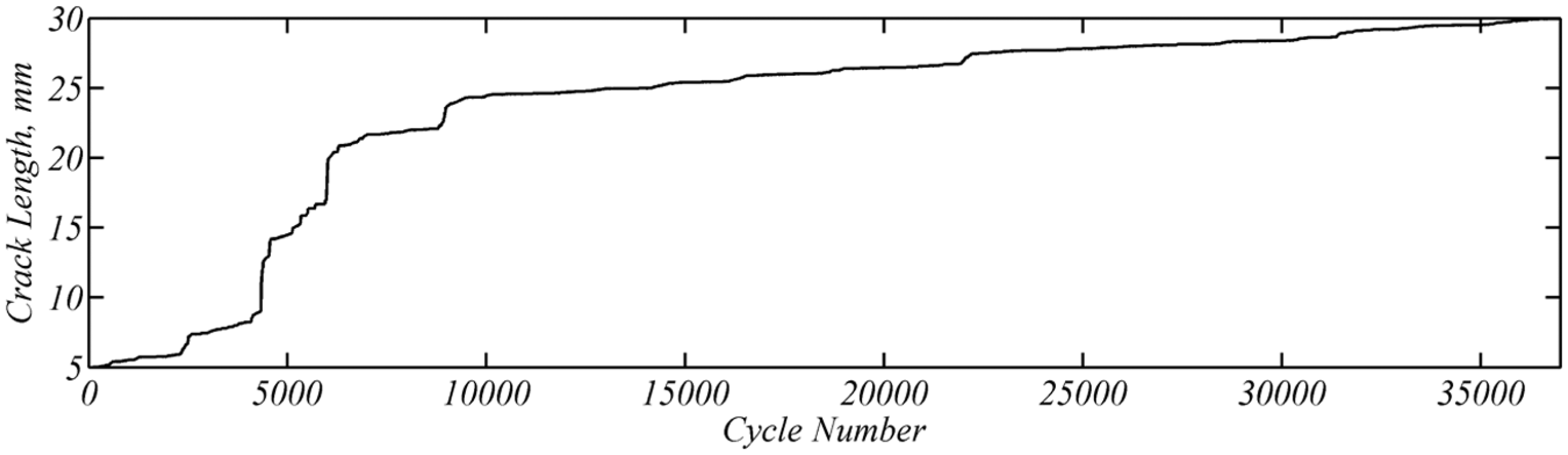
Comparison of the crack size as a function of the cycle number.

One of the observations from Figure 10 is that most of the crack growth occurs early in the cyclic loading history for the wing panel. In Figure 11, the stress intensity factor range as a function of cycle number is given, along with the threshold stress intensity factor range. Note that the equivalent ΔK in Figure 11 rarely exceeds the threshold stress intensity factor range. This can be explained by the artificial stress scaling which was done to promote fatigue crack growth. It should also be noted that early in the life of the plate (in particular before 10,000 cycles), there is a high concentration of ΔK which exceeds ΔK_th. This results in increased crack growth in Figure 10 early in the life of the plate, compared to later when ΔK rarely exceeds ΔK_th.

Figure 11.

Stress intensity factor range as a function of the cycle number.

The path of crack growth is shown in Figure 12, which corresponds to the crack growth and ΔK curves of Figures 10 and 11. The location of the crack tip at discrete cycle number is given where the crack tip location is denoted with small data points. As we would expect, most of the crack growth occurs before reaching the cycle number 10,000. It can be noted from Figure 5 that, in general, the stress components can be ordered in decreasing magnitude as σ_yy, σ_xy, and σ_xx. Therefore, it could be expected that the general trend of crack growth would be horizontal, with some deviation according to the values of σ_xy and σ_xx, which is the behavior shown in Figure 12.

Figure 12.

Predicted crack path under non-proportional bi-axial variable amplitude loading.

Conclusion and future work

In this article, usage monitoring data from an aircraft were converted into a stress history through the use of simple analysis to predict the magnitude of the lift and drag pressure distributions upon a wing box. A combination of finite element analysis for the wing box and surrogate models was used to convert the magnitudes of the lift and drag pressure distributions into bi-axial stress histories for a point of interest along the wing box.

A fatigue crack growth analysis was then performed using a modified Paris model to consider the effects of variable amplitude loading and the critical plane approach to determine the crack growth direction. For calculation, XFEM was implemented where the changes in the stiffness matrix are handled by direct modification of an existing factorization to handle the large number of required simulations. It would be challenging for a classical finite element approach to handle the number of simulations and the corresponding evolution of the finite element mesh.

This work should be viewed as a means to (a) approximate the service stress history from usage monitoring data and (b) estimate the remaining life of a structure according to a service history. The service stress history could also be used as the input into a prognosis method, which often assumes that a service stress history, or at least an estimate of the service stress history, is available. In the future, the combination of prognosis methods with estimates of the future crack growth provided by numerical simulations for the service stress history may lead to a more robust prediction of the remaining useful life.