A fractional model to describe the Brownian motion of particles and its analytical solution

Abstract

In this article, we apply a relatively modified analytic iterative method for solving a time-fractional Fokker–Planck equation subject to given constraints. The utilized method is a numerical technique based on the generalization of residual error function and then applying the generalized Taylor series formula. This method can be used as an alternative to obtain analytic solutions of different types of fractional partial differential equations such as Fokker–Planck equation applied in mathematics, physics, and engineering. The solutions of our equation are calculated in the form of a rapidly convergent series with easily computable components. The validity, potentiality, and practical usefulness of the proposed method have been demonstrated by applying it to several numerical examples. The results reveal that the proposed methodology is very useful and simple in determination of solution of the Fokker–Planck equation of fractional order.

Introduction

In this article, a sincere attempt has been taken to solve the nonlinear Riesz time-fractional Fokker–Planck equation (FPE) of the form

$${}_0^{\Re }{D}_t^{\alpha }u(x,t)=[-D_{x}A(x,t,u)+D_x^{2}B(x,t,u)]u(x,t)$$

(1)

with the initial condition given by ${\partial }^{j}u(x,t_0)/\partial t^j={\varphi }_j(x),x\in R,j=0,1,2,\dots ,m-1$ , where ${}_0^{\Re }{D}_t^{\alpha }$ is the Riesz time-fractional derivative of order $\alpha$ , ${\varphi }_j(x)$ is given analytic function on $R$ . In the whole article, $N$ is the set of natural numbers, $R$ is the set of real numbers, and $\Gamma$ is the gamma function. $A(x,t,u)$ and $B(x,t,u)$ are drift and diffusion coefficients, respectively. Here, $\alpha$ is the parameter representing the order of fractional derivatives, which satisfies $m-1<\alpha \le m$ , and $t>0$ . When $\alpha =1$ , the fractional equation reduces to the classical FPE.

FPE was introduced by Fokker and Planck, ¹ which is a mathematical model that arises in a wide variety of natural science, including solid-state physics, quantum optics, chemical physics, theoretical biology, and circuit theory. It has been commonly used to describe the Brownian motion of particles as well as the change of probability of a random function in space and time. Applications of FPE are widely in different branches of sciences and technology such as plasma physics, surface physics, population dynamics, biophysics, neuroscience, nonlinear hydrodynamics, pattern formation, psychology, and marketing. ² In recent past, Yildirim ³ and Kumar ⁴ have given the numerical and analytical approximate solutions of the FPE using homotopy perturbation method^5–7 and homotopy perturbation transform method,^8,9 respectively.

Recently, the authors used some novel method to solve fractional differential equations (FDEs). ¹⁰ For other application of FDEs in the field of engineering, especially mechanics, see Yang et al. ¹¹ In this present analysis, we employ a relatively modified approach residual power series method (RPSM) to find an analytical and approximate solution of FPE. The RPSM^12,13 is effective and easy for constructing power series expansion solutions for nonlinear equations of different types and orders without linearization, perturbation, or discretization. The main advantage of this method is the obtained solutions, and all their fractional derivatives are applicable for each arbitrary point and multidimensional variables in the given domain by choosing an appropriate initial guess approximation. Regarding the other aspect, the RPSM does not require any conversion while switching from the low order to the higher order and from simple linearity to complex nonlinearity.

The rest of this article is organized as follows: In the next section, we utilize some basic definitions of fractional calculus and theorem of power series expansions. In section “Construction of RPSM,” basic idea of the RPSM and its convergence analysis is presented. To determine the approximate solution for the Riesz time-fractional FPE, RPSM has been applied in section “Applications and numerical discussions.” Finally, section “Conclusion” concludes the whole article.

Mathematical preliminaries of fractional calculus and fractional power series

This section describes operational properties for elucidating sufficient fractional calculus theory, to enable us to follow the solutions of Riesz time-fractional FPE. In recent year, the FDEs have gained much attention due to the fact that they generate fractional Brownian motion, which is generalization of Brownian motion.^14,15

Definition 1

A real function $u(x,t)$ is said to be in the space $C_{\mu },\mu \in R$ if there exists a real number $p(>\mu )$ , such that $u(x,t)=x^p{u}_1(x,t)$ , where $u_1(x,t)\in C[0,\infty )$ , and it is said to be in the space $C_{\mu }^m$ if and only if $u^{(m)}\in C_{\mu },m\in N$ .

Definition 2

The Reimann–Liouville fractional integral operator of the order $m-1<\alpha \le m$ of a function $u(x,t)\in C_{\mu }$ , $\mu \ge -1$ , is defined as^14,15

$$\underset{t}{\overset{\alpha }{\int }}u(x,t)=\frac{1}{\Gamma \left(\alpha \right)}\underset{0}{\overset{t}{\int }}{(t-\zeta )}^{\alpha -1}u(x,\zeta )d\zeta ,t>0,\alpha \in R^{+}$$

where $R^{+}$ is the set of positive real numbers.

Definition 3

The Riesz fractional derivative of the order $m-1<\alpha \le m$ of a function $u(x,t)\in C_{\mu }$ , $\mu \ge -1$ , is defined as^14–16

$${}_0^{\Re }{D}_t^{\alpha }u(x,t)=-c_{\alpha }({}_0{D}_t^{\alpha }+{}_t{D}_{t_0}^{\alpha })u(x,t)$$

where $-c_{\alpha }=(1/2)\cos (\pi \alpha /2)$ , $\alpha \ne 1$ , and ${}_0{D}_t^{\alpha }\mathrm{and}{}_t{D}_{t_0}^{\alpha }$ are the left- and right-hand side Reimann–Liouville fractional operators, respectively.

Definition 4

For $0\le m-1<\alpha \le m$ , a power series of the form ¹²

$$\sum _{i=0}^{\infty }\sum _{j=0}^{m-1}{f}_{\mathrm{ij}}\left(x\right){(t-t_0)}^{i\alpha +j},t\ge t_0$$

is called a multiple fractional power series (FPS) about $t=t_0$ , where $t$ is a variable and $f_{\mathrm{ij}}(x)$ are functions of $x$ called the coefficients of the series.

Theorem 1

Suppose that $f$ has a FPS representation at $t=t_0$ of the form ¹²

$$\sum _{i=0}^{\infty }\sum _{j=0}^{m-1}{c}_{\mathrm{ij}}\left(x\right){(t-t_0)}^{i\alpha +j},0\le m-1<\alpha \le m,t_0\le t<t_0+R$$

Furthermore, if $D^{i\alpha +j}f(t)$ are continuous on $(t_0,t_0+R),n=0,1,2,\dots ,$ then the coefficient $c_{\mathrm{ij}}$ is given by the following formula

$$c_{\mathrm{ij}}=\frac{D^{i\alpha +j}f\left(t_0\right)}{\Gamma (i\alpha +j+1)},i=0,1,2,\dots$$

where $D^{i\alpha }=D^{\alpha },D^{\alpha },\dots ,D^{\alpha }$ ( $i$ times) and $R$ is the radius of convergence.

Construction of RPSM

In this section, we construct and obtain solution of fractional FPE by substituting its FPS expansion among its truncated residual function. From the resulting equation, a recursion formula for the computation of the coefficients is derived, while the coefficients in the FPS expansion can be computed recursively by recurrent fractional differentiation of the truncated residual function.

The RPSM consists in expression of the solution of equation (1) as multiple FPS expansions about the initial point $t=t_0$ . Let us consider the following form of the solution

$$\begin{array}{c}\multicolumn{1}{c}{u(x,t)=\sum _{i=0}^{\infty }\sum _{j=0}^{m-1}{f}_{\mathrm{ij}}\left(x\right)\frac{{(t-t_0)}^{i\alpha +j}}{\Gamma (i\alpha +j+1)},}\\ \multicolumn{1}{c}{m-1<\alpha \le m,x\in R,0\le t<R}\end{array}$$

(2)

In fact, $u(x,t)$ satisfies the initial conditions of equation (1), so from equation (2), we obtain ${\partial }^{j}u(x,t_0)/\partial t^j=j!f_{0j}(x)={\varphi }_j(x),j=0,1,2,\dots ,m-1$ . Then, $f_{0j}(x)={\varphi }_j(x)/j!,j=0,1,2,\dots ,m-1$ , and the initial guess approximation of $u(x,t)$ can be written as

$$\begin{array}{c}\multicolumn{1}{c}{u_{(0,m-1)}(x,t)=\sum _{j=0}^{m-1}\frac{{\varphi }_j\left(x\right)}{j!}{(t-t_0)}^j,}\\ \multicolumn{1}{c}{x\in R,t_0\le t<t_0+R}\end{array}$$

(3)

With the help of equation (3), we can reformulate the expansion form of equation (2) as follows

$$\begin{array}{c}\multicolumn{1}{c}{u(x,t)=\sum _{j=0}^{m-1}\frac{{\varphi }_j\left(x\right)}{j!}{(t-t_0)}^j+\sum _{i=1}^{\infty }\sum _{j=0}^{m-1}{f}_{\mathrm{ij}}\left(x\right)\frac{{(t-t_0)}^{i\alpha +j}}{\Gamma (i\alpha +j+1)},}\\ \multicolumn{1}{c}{x\in R,t_0\le t<t_0+R}\end{array}$$

(4)

The RPSM provides an analytical approximate solution in terms of an infinite multiple FPS. However, to obtain numerical values from this series, the consequent series truncation and the practical procedure are conducted to accomplish this task. In the following step, we will let $u_{(k,l)}(x,t)$ to denote the (k, l)-truncated series of $u(x,t)$ . That is

$$\begin{array}{c}\multicolumn{1}{c}{u_{(k,l)}(x,t)=\sum _{j=0}^{m-1}\frac{{\varphi }_j\left(x\right)}{j!}{(t-t_0)}^j+\sum _{i=1}^k\sum _{j=0}^l{f}_{\mathrm{ij}}\left(x\right)\frac{{(t-t_0)}^{i\alpha +j}}{\Gamma (i\alpha +j+1)},}\\ \multicolumn{1}{c}{x\in R,t\ge t_0}\end{array}$$

(5)

where the indices counters $k=1,2,3,\dots$ and $l=0,1,2,3,\dots ,m-1$ .

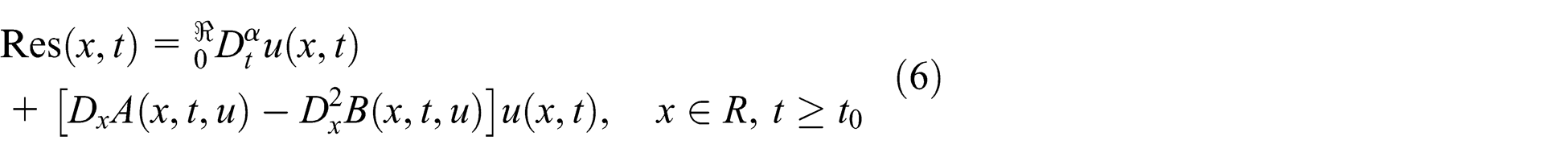
According to RPSM, for finding the coefficients $f_{\mathrm{ij}}(x)$ in the series expansion of equation (5), we must define the residual function concept for equation (1) as

$$\begin{array}{c}\multicolumn{1}{c}{\mathrm{Res}(x,t){=}_0^{\Re }{D}_t^{\alpha }u(x,t)}\\ \multicolumn{1}{c}{+[D_{x}A(x,t,u)-D_x^{2}B(x,t,u)]u(x,t),x\in R,t\ge t_0}\end{array}$$

(6)

and the following (k, l)-truncated residual function

$$\begin{array}{c}\multicolumn{1}{c}{\mathrm{Re}{\mathrm{s}}_{(k,l)}(x,t){=}_0^{\Re }{D}_t^{\alpha }{u}_{(k,l)}(x,t)}\\ \multicolumn{1}{c}{+[D_{x}A(x,t,u)-D_x^{2}B(x,t,u)]u_{(k,l)}(x,t),x\in R,t\ge t_0}\end{array}$$

(7)

As described in El-Ajou et al. ¹² and Abu Arqub et al., ¹³ it is clear that $\mathrm{Res}(x,t)=0$ for each $t\in [t_0,t_0+R),x\in R$ , where $R$ is a nonnegative real number. In fact, this shows that ${}_0^{\Re }{D}_t^{(i-1)}{}^{\alpha }{}_0^{\Re }{D}_t^j\mathrm{Res}(x,t)=0$ for each $i=1,2,3,\dots ,k$ and $j=0,1,2,3,\dots ,l$ , since the Riesz fractional derivative of a constant function is zero. Again, the fractional derivatives ${}_0^{\Re }{D}_t^{(i-1)}{}^{\alpha }{}_0^{\Re }{D}_t^j$ for each $i=1,2,3,\dots ,k$ and $j=0,1,2,3,\dots ,l$ of $\mathrm{Res}(x,t)$ and $\mathrm{Re}{\mathrm{s}}_{(i,j)}(x,t)$ are matching at $(x,t)=(x,t_0)$ . Therefore, we have the following equation

$${}_0^{\Re }{D}_t^{(i-1)\alpha }{}_0^{\Re }{D}_t^j\mathrm{Re}s\left(x,t\right){=}_0^{\Re }{D}_t^{(i-1)\alpha }{}_0^{\Re }{D}_t^j\mathrm{Re}{s}_{(i,j)}\left(x,t\right)=0,x\in R,i=1,2,3,\dots ,k,j=0,1,2,\dots ,l$$

(8)

To obtain the coefficients $f_{\mathrm{vw}}$ in equation (7), we can apply the following subroutine: substitute (v, w)-truncated series of $u(x,t)$ into equation (7), find the fractional derivative formula $D_t^{(v-1)\alpha }{D}_t^w$ of ${\mathrm{Res}}_{(v,w)}(x,t)$ at $t=t_0$ , and then finally solve the obtained algebraic equation.

To summarize the computation process of RPSM in numerical values, we apply the following steps: at first, fix $i=1$ and run the counter $j=0,1,2,\dots ,l$ to find (1, j)-truncated series expansion of suggested solution, and next, fix $i=2$ and run the counter $j=0,1,2,\dots ,l$ to find (2, j)-truncated series and so on. Here, to find (1, 0)-truncated series expansion of equation (1), we use equation (5) and write

$$\begin{array}{c}\multicolumn{1}{c}{u_{(1,0)}(x,t)={\varphi }_0\left(x\right)+{\varphi }_1\left(x\right)(t-t_0)+\cdots +{\varphi }_{m-1}\left(x\right)}\\ \multicolumn{1}{c}{\frac{{(t-t_0)}^{(m-1)}}{(m-1)!}+f_{10}\left(x\right)\frac{{(t-t_0)}^{\alpha }}{\Gamma (\alpha +1)}}\end{array}$$

(9)

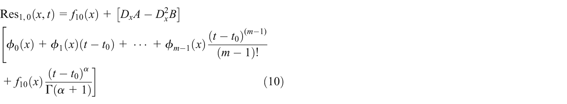
For finding the first unknown coefficient $f_{10}(x)$ in equation (9), we should substitute equation (9) into both sides of the $(1,0)$ residual function that was obtained from equation (7), to obtain the following result

$$\begin{array}{c}\multicolumn{1}{c}{\mathrm{Re}{\mathrm{s}}_{1,0}(x,t)=f_{10}\left(x\right)+[D_{x}A-D_x^{2}B]}\\ \multicolumn{1}{c}{[{\varphi }_0\left(x\right)+{\varphi }_1\left(x\right)(t-t_0)+\cdots +{\varphi }_{m-1}\left(x\right)\frac{{(t-t_0)}^{(m-1)}}{(m-1)!}}\\ \multicolumn{1}{c}{+f_{10}\left(x\right)\frac{{(t-t_0)}^{\alpha }}{\Gamma (\alpha +1)}]}\end{array}$$

(10)

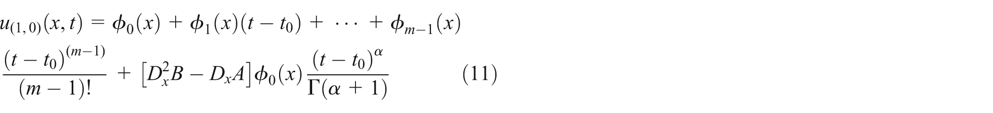
Depending on the result of equation (8) for $(i,j)=(1,0)$ , equation (10) gives $f_{10}(x)=[D_x^{2}B-D_{x}A]{\varphi }_0(x)$ . Hence, using the (1, 0)-truncated series expansion of equation (9), the (1, 0) residual power series (RPS) approximate solution for equation (1) can be expressed as

$$\begin{array}{c}\multicolumn{1}{c}{u_{(1,0)}(x,t)={\varphi }_0\left(x\right)+{\varphi }_1\left(x\right)(t-t_0)+\cdots +{\varphi }_{m-1}\left(x\right)}\\ \multicolumn{1}{c}{\frac{{(t-t_0)}^{(m-1)}}{(m-1)!}+[D_x^{2}B-D_{x}A]{\varphi }_0\left(x\right)\frac{{(t-t_0)}^{\alpha }}{\Gamma (\alpha +1)}}\end{array}$$

(11)

Similarly, to find out the (2, 0)-truncated series expansion for equation (1), we use equation (5) and write

$$\begin{array}{c}\multicolumn{1}{c}{u_{(2,0)}(x,t)={\varphi }_0\left(x\right)+{\varphi }_1\left(x\right)(t-t_0)+\cdots +{\varphi }_{m-1}\left(x\right)\frac{{(t-t_0)}^{(m-1)}}{(m-1)!}}\\ \multicolumn{1}{c}{+[D_x^{2}B-D_{x}A]{\varphi }_0\left(x\right)\frac{{(t-t_0)}^{\alpha }}{\Gamma (\alpha +1)}+f_{20}\left(x\right)\frac{{(t-t_0)}^{\alpha +1}}{\Gamma (\alpha +2)}}\end{array}$$

(12)

Again, to find out the form of the second unknown coefficient $f_{20}(x)$ in equation (12), we must find and formulate (2, 0) residual function based on equation (7) and then substitute the form of $u_{(2,0)}(x,t)$ of equation (12) to find new discretized form of this residual function as follows

$$\begin{array}{c}\multicolumn{1}{c}{\mathrm{Re}{\mathrm{s}}_{(2,0)}(x,t)=f_{10}\left(x\right)+f_{20}\left(x\right)(t-t_0)+[D_{x}A-D_x^{2}B]}\\ \multicolumn{1}{c}{[{\varphi }_0\left(x\right)+{\varphi }_1\left(x\right)(t-t_0)+\cdots +{\varphi }_{m-1}\left(x\right)\frac{{(t-t_0)}^{(m-1)}}{(m-1)!}}\\ \multicolumn{1}{c}{+[D_x^{2}B-D_{x}A]{\varphi }_0\left(x\right)\frac{{(t-t_0)}^{\alpha }}{\Gamma (\alpha +1)}+f_{20}\left(x\right)\frac{{(t-t_0)}^{\alpha +1}}{\Gamma (\alpha +2)}]}\end{array}$$

(13)

By considering equation (8) for $(i,j)=(2,0)$ and applying the operator ${}_0^{\Re }{D}_t^{\alpha }$ on both sides of equation (13), we obtain

$${}_0^{\Re }{D}_t^{\alpha }\mathrm{Re}{s}_{(2,0)}\left(x,t\right)=f_{20}\left(x\right){+}_0^{\Re }{D}_t^{\alpha }\left[\left[D_{x}A-D_x^{2}B\right]\left[{\varphi }_0\left(x\right)+{\varphi }_1\left(x\right)\left(t-t_0\right)+\cdots +{\varphi }_{m-1}\left(x\right)\frac{{\left(t-t_0\right)}^{(m-1)}}{\left(m-1\right)!}+\left[D_x^{2}B-D_{x}A\right]{\varphi }_0\left(x\right)\frac{{\left(t-t_0\right)}^{\alpha }}{\Gamma \left(\alpha +1\right)}+f_{20}\left(x\right)\frac{{\left(t-t_0\right)}^{\alpha +1}}{\Gamma \left(\alpha +2\right)}\right]\right]$$

(14)

Using the fact that ${}_0^{\Re }{D}_t^{(i-1)}{}^{\alpha }{}_0^{\Re }{D}_t^j\mathrm{Res}(x,t_0)=0$ for $(i,j)=(2,0)$ from equation (8) and solving the resultant algebraic equation for $f_{20}(x)$ , we obtain

$$f_{20}\left(x\right)={[D_x^{2}B-D_{x}A]}^2{\varphi }_0\left(x\right)+[D_x^{2}B-D_{x}A]{\varphi }_1\left(x\right)$$

(15)

Hence, using the (2, 0)-truncated series expansion of equation (2), the $(2,0)$ RPS approximate solution for equation (1) can be expressed as

$$\begin{array}{c}\multicolumn{1}{c}{u_{(2,0)}(x,t)={\varphi }_0\left(x\right)+{\varphi }_1\left(x\right)(t-t_0)+\cdots +{\varphi }_{m-1}\left(x\right)}\\ \multicolumn{1}{c}{\frac{{(t-t_0)}^{(m-1)}}{(m-1)!}+[D_x^{2}B-D_{x}A]{\varphi }_0\left(x\right)\frac{{(t-t_0)}^{\alpha }}{\Gamma (\alpha +1)}}\\ \multicolumn{1}{c}{+[{[D_x^{2}B-D_{x}A]}^2{\varphi }_0\left(x\right)+[D_x^{2}B-D_{x}A]{\varphi }_1\left(x\right)]}\\ \multicolumn{1}{c}{\frac{{(t-t_0)}^{\alpha +1}}{\Gamma (\alpha +2)}}\end{array}$$

(16)

This procedure can be repeated till the arbitrary order coefficients of the multiple FPS solution of equation (1) are obtained. But if there is a pattern in the series coefficients, then calculating few of the terms in series is sufficient to reach the solution.

In this part, we study the convergence of RPS through the given theorem.

Theorem 2

Suppose that $u(x,t)$ has a FPS representation of the form $u(x,t)=\sum _{i=0}^{\infty }\sum _{j=0}^{m-1}{f}_{\mathrm{ij}}(x)t^{i\alpha +j},0\le m-1<\alpha \le m$ , and $\mathrm{limsup}{\left|f_{\mathrm{ij}}\right|}^{1/(i\alpha +j)}=\mu$ . Then, we have

1. If $\mu =0$ , the series is everywhere convergent;

2. If $0<\mu <\infty$ , the series is absolutely convergent for all $t$ satisfying $\left|t\right|<1/\mu$ and is divergent for all $t$ satisfying $\left|t\right|>1/\mu$ ;

3. If $\mu =\infty$ , the series is nowhere convergent.

Proof 1

1. Let $k_0\ne 0$ and $ϵ=1/2\left|k_0\right|$ . Since $\mathrm{limsup}{\left|f_{\mathrm{ij}}\right|}^{1/(i\alpha +j)}=0$ , there exist a natural number k such that ${\left|f_{\mathrm{ij}}\right|}^{1/(i\alpha +j)}<ϵ$ for all $i,j\ge k$ or $\left|f_{\mathrm{ij}}{k}_0^{i\alpha +j}\right|<1/2^{i\alpha +j}$ for all $i,j\ge k$ . Since $\sum _{i=0}^{\infty }\sum _{j=0}^{m-1}1/2^{i\alpha +j}$ is a convergent series of positive terms, by comparison test, $\sum _{i=0}^{\infty }\sum _{j=0}^{m-1}\left|f_{\mathrm{ij}}{k}_0^{i\alpha +j}\right|$ is also convergent series. It follows that $\sum _{i=0}^{\infty }\sum _{j=0}^{m-1}{f}_{\mathrm{ij}}{k}_0^{i\alpha +j}$ is absolutely convergent and hence convergent. As $k_0$ is arbitrary, the series $\sum _{i=0}^{\infty }\sum _{j=0}^{m-1}{f}_{\mathrm{ij}}{t}^{i\alpha +j}$ is everywhere convergent.

2. $\mathrm{limsup}(\sqrt[i\alpha +j]{\left|f_{\mathrm{ij}}{t}^{i\alpha +j}\right|})=\mathrm{limsup}(\sqrt[i\alpha +j]{\left|f_{\mathrm{ij}}\right|}\left|t\right|)=\left|t\right|\mu$ . By Cauchy’s root test, the series $\sum _{i=0}^{\infty }\sum _{j=0}^{m-1}\left|f_{\mathrm{ij}}{t}^{i\alpha +j}\right|$ is convergent if $\left|t\right|\mu <1$ . Therefore if $\left|t\right|<1/\mu$ , the series $\sum _{i=0}^{\infty }\sum _{j=0}^{m-1}\left|f_{\mathrm{ij}}{t}^{i\alpha +j}\right|$ is convergent, that is, the series $\sum _{i=0}^{\infty }\sum _{j=0}^{m-1}{f}_{\mathrm{ij}}{t}^{i\alpha +j}$ is absolutely convergent. If $\left|t\right|\mu <1$ , $\mathrm{limsup}(\sqrt[i\alpha +j]{\left|f_{\mathrm{ij}}{t}^{i\alpha +j}\right|})=\mathrm{limsup}(\sqrt[i\alpha +j]{\left|f_{\mathrm{ij}}\right|}\left|t\right|)>1$  =  $\mathrm{limsup}(\sqrt[i\alpha +j]{\left|f_{\mathrm{ij}}\right|}\left|t\right|)>1$ . Let $v_{\mathrm{ij}}=f_{\mathrm{ij}}{t}^{i\alpha +j}$ . Then, $\mathrm{limsup}\left|v_{\mathrm{ij}}\right|>1$ , and this implies $\lim \left|v_{\mathrm{ij}}\right|\ne 0$ . Consequently, $\lim \left|v_{\mathrm{ij}}\right|\ne 0$ , and it follows that $\sum _{i=0}^{\infty }\sum _{j=0}^{m-1}{v}_{\mathrm{ij}}$ is divergent.

3. If possible, let the series $\sum _{i=0}^{\infty }\sum _{j=0}^{m-1}{f}_{\mathrm{ij}}{t}^{i\alpha +j}$ be convergent for $t=k_0,(k_0\ne 0)$ . Then, $\lim f_{\mathrm{ij}}{k}_0^{i\alpha +j}=0$ . The sequence $\{f_{\mathrm{ij}}{k}_0^{i\alpha +j}\}$ being a bounded sequence, there exists a positive real number B such that $\left|f_{\mathrm{ij}}{k}_0^{i\alpha +j}\right|<B$ for all $i,j\in N$ . This shows that the sequence $\{{\left|f_{\mathrm{ij}}\right|}^{1/(i\alpha +j)}\}$ is bounded sequence, and this contradicts that $\mathrm{limsup}{\left|f_{\mathrm{ij}}\right|}^{1/(i\alpha +j)}=\infty$ . Thus, the series $\sum _{i=0}^{\infty }\sum _{j=0}^{m-1}{f}_{\mathrm{ij}}{t}^{i\alpha +j}$ is not convergent for $t=k_0$ . As $k_0$ is arbitrary nonzero real number, the series $\sum _{i=0}^{\infty }\sum _{j=0}^{m-1}{f}_{\mathrm{ij}}{t}^{i\alpha +j}$ is nowhere convergent.

Applications and numerical discussions

The application problems are carried out using the proposed RPSM, which is one of the modern analytical techniques because of its iteratively nature. In this section, we consider the time-fractional FPE to show potentiality, generality, and efficiency of our method. Throughout this work, all the symbolic and numerical computations were performed by using MATHEMATICA 7 software package.

Example 1

Consider the following time-fractional FPE ⁴

$${}_0^{\Re }{D}_t^{\alpha }u=-D_x\left(\mathrm{xu}\right)+D_x^2\left(\frac{x^{2}u}{2}\right)x,t>0,0<\alpha \le 1$$

(17)

with the initial condition $u(x,0)=x$ . The exact solution of the problem is given by $u(x,t)=x{e}^t$ for $\alpha =1$ . According to equation (4) with ${\varphi }_0(x)=x$ , and considering $A(x,t,u)=x$ and $B(x,t,u)=x^2/2$ , the series solution of equation (17) can be written as

$$u(x,t)=x+\sum _{i=1}^{\infty }{f}_{i0}\left(x\right)\frac{{\left(t\right)}^{i\alpha }}{\Gamma (i\alpha +1)}$$

(18)

where $u_{0,0}(x,t)=x$ is the initial guess approximation which is obtained directly from equation (3). Next, according to equations (5) and (7), the (k, 0)-truncated series of $u(x,t)$ and the (k, 0)-truncated residual function of equation (17) can be defined and thus constructed, respectively, as follows

$$\begin{array}{c}\multicolumn{1}{c}{u_{(k,l)}(x,t)=x+\sum _{i=1}^{\infty }{f}_{i0}\left(x\right)\frac{{\left(t\right)}^{i\alpha }}{\Gamma (i\alpha +1)},}\\ \multicolumn{1}{c}{k=1,2,3,\dots ,l=0}\end{array}$$

(19)

$$\begin{array}{c}\multicolumn{1}{c}{\mathrm{Re}{\mathrm{s}}_{(k,l)}(x,t){=}_0^{\Re }{D}_t^{\alpha }{u}_{(k,l)}(x,t)+\frac{\partial \left(x{u}_{(k,l)}\right)}{\partial x}-\frac{{\partial }^2\left(\frac{x^2{u}_{(k,l)}(x,t)}{2}\right)}{\partial x^2},}\\ \multicolumn{1}{c}{k=1,2,3,\dots ,l=0}\end{array}$$

(20)

To determine the form of coefficient $f_{10}(x)$ , in the expansion of equation (19), we should substitute the (1, 0)-truncated series $u_{(1,0)}(x,t)=x+f_{10}(x)(t^{\alpha }/\Gamma (1+\alpha ))$ into the (1, 0)-truncated residual function $\mathrm{Re}{\mathrm{s}}_{(1,0)}(x,t){=}_0^{\Re }{D}_t^{\alpha }{u}_{(1,0)}(x,t)+(\partial (x{u}_{(1,0)})/\partial x)-({\partial }^2((x^2{u}_{(1,0)}(x,t))/2)/\partial x^2$ to obtain

$$\mathrm{Re}{\mathrm{s}}_{(1,0)}(x,t)=f_{(10)(x)}-x$$

(21)

Depending on the results of equation (8) in case of $(i,j)=(1,0)$ , one can obtain $f_{10}(x)=x$ . Hence, the (1, 0)-truncated series solution of equation (17) could be expressed as

$$u_{(1,0)}(x,t)=x+x\frac{t^{\alpha }}{\Gamma (1+\alpha )}$$

(22)

Again, to find out the form of the second unknown coefficient $f_{20}(x)$ , we substitute the (2, 0)-truncated series solution $u_{(2,0)}(x,t)=x+x(t^{\alpha }/\Gamma (1+\alpha ))+f_{20}(x)(t^{2\alpha }/\Gamma (1+2\alpha ))$ into the (2, 0)-truncated residual function $\mathrm{Re}{\mathrm{s}}_{(2,0)}(x,t){=}_0^{\Re }{D}_t^{\alpha }{u}_{(2,0)}(x,t)+(\partial (x{u}_{(2,0)})/\partial x)-({\partial }^2(x^2{u}_{(2,0)}(x,t)/2)/\partial x^2)$ to obtain

$$\mathrm{Re}{\mathrm{s}}_{(2,0)}(x,t)=f_{20}\left(x\right)\frac{t^{\alpha }}{\Gamma (1+\alpha )}-x\frac{t^{\alpha }}{\Gamma (1+\alpha )}$$

(23)

Now, applying the operator ${}_0^{\Re }{D}_t^{\alpha }$ one time on both sides of equation (23) and according to equation (8) for $(i,j)=(2,0)$ , we have $f_{20}(x)=x$ . Therefore, the (2, 0)-truncated series solution of equation (17) is obtained, and one can collect the previous results to obtain the following expansion

$$u_{(2,0)}(x,t)=x+x\frac{t^{\alpha }}{\Gamma (1+\alpha )}+x\frac{t^{2\alpha }}{\Gamma (1+2\alpha )}$$

(24)

As the former, by applying the same procedure for $(i,j)$ , $i=2,3,4,\dots$ and $j=0$ will yield after easy calculations to $f_{\mathrm{ij}}(x)=x$ . Furthermore, if we collect all the final results, then the RPS solution of equation (17) can be constructed in the form of infinite series as follows

$$\begin{array}{c}\multicolumn{1}{c}{u(x,t)=}\\ \multicolumn{1}{c}{x(1+\frac{t^{\alpha }}{\Gamma (1+\alpha )}+\frac{t^{2\alpha }}{\Gamma (1+2\alpha )}+\frac{t^{3\alpha }}{\Gamma (1+3\alpha )}+\cdots )}\\ \multicolumn{1}{c}{=x\sum _{k=0}^{\infty }\frac{t^{k\alpha }}{\Gamma (1+k\alpha )}=x{E}_{\alpha }\left(t^{\alpha }\right)}\end{array}$$

(25)

where $E_{\alpha }(t^{\alpha })=\sum _{k=0}^{\infty }(t^{k\alpha }/\Gamma (1+k\alpha )),\alpha >0$ , is the Mittag-Leffler function in one parameter. As a special case when $\alpha =1$ , the RPS solution of equation (17) has the general pattern form which coincides with the exact solution of the standard FPE in terms of infinite series

$$u(x,t)=x(1+t+\frac{t^2}{2!}+\frac{t^3}{3!}+\frac{t^4}{4!}+\cdots ))=x{e}^t$$

(26)

The above result is completely in agreement with the Yildirim ³ and Kumar. ⁴

The geometric behavior of the solutions of equation (17) is studied next in Figure 1 by drawing the three-dimensional space figures of the (4, 0)-truncated series solution together with the exact solution on the domain $[0,2]\times [0,2]$ . It is clear from the scenario of Figure 1 that Figure 1(a)–(d) is nearly coinciding and similar in behavior. Again to show the accuracy of the RPSM, we report absolute error in Figure 1(e). Of course, the accuracy can be improved by computing further terms of the approximate solutions using the present methods.

Figure 1.

(a) Exact solution $u(x,t)$ for equation (17), (b) the surface graph of the RPS approximation solution $u_{(4,0)}(x,t)$ for equation (17) when $\alpha =1$ , (c) the surface graph of the RPS approximation solution $u_{(4,0)}(x,t)$ for equation (17) when $\alpha =0.75$ , (d) the surface graph of the RPS approximation solution $u_{(4,0)}(x,t)$ for equation (17) when $\alpha =0.50$ , and (e) absolute error $E_{(4,0)}(h)=|u(x,t)-u_{(4,0)}(x,t)|$ .

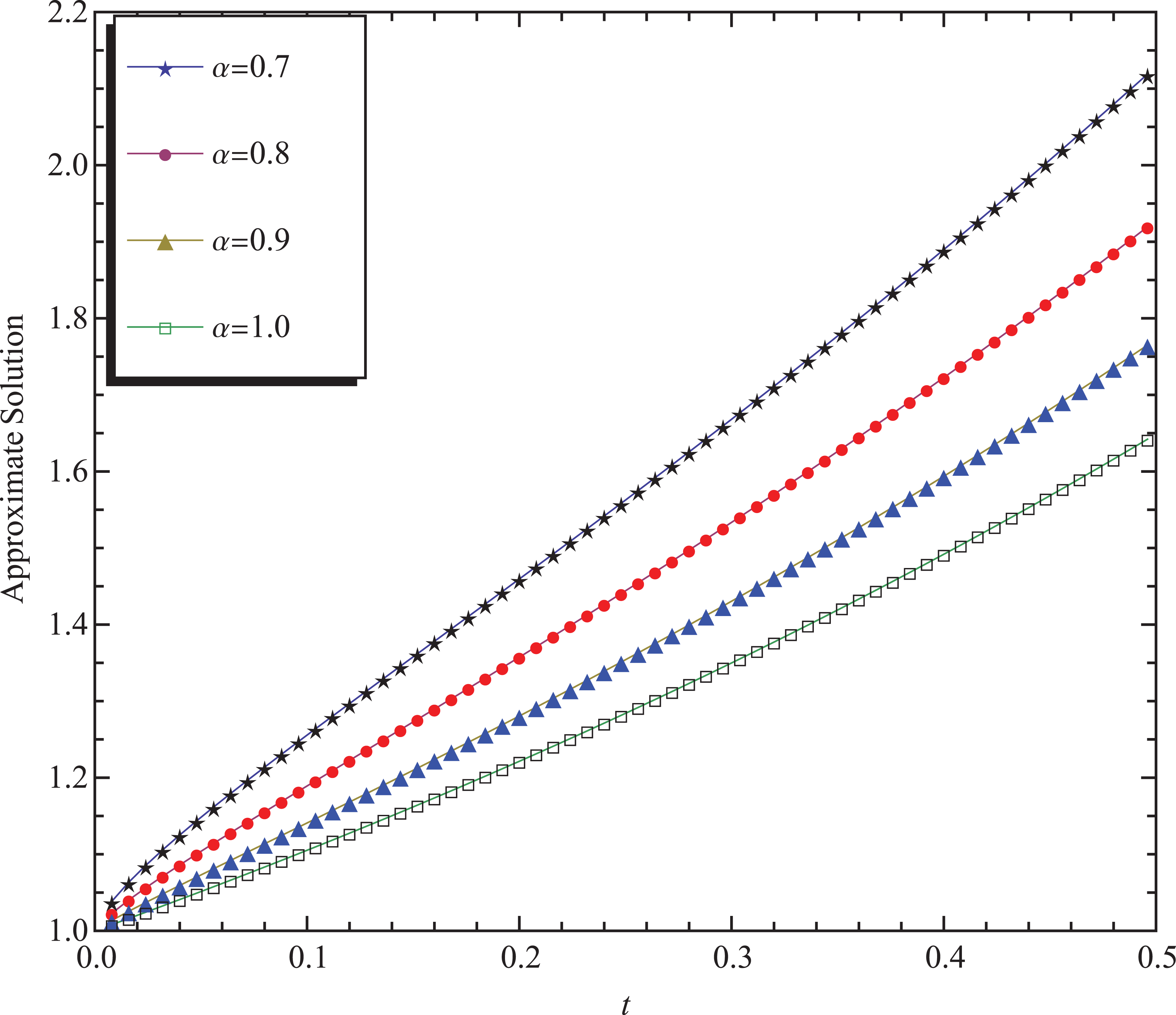
Figure 2 shows the evaluation results of the approximate analytical solution of equation (17) obtained by the RPSM for different fractional Brownian motions, that is, $\alpha =0.7,\alpha =0.8,\mathrm{and}\alpha =0.9$ , and standard motions, that is, $\alpha =1$ . Our solutions obtained by the proposed methods increase very rapidly with the increase in $t$ at $x=1$ .

Figure 2.

Plot of $u_4(x,t)$ versus time $t$ for different value of $\alpha$ at x = 1.

Example 2

Consider the following time-fractional FPE ⁴

$${}_0^{\Re }{D}_t^{\alpha }u=-D_x\frac{\mathrm{xu}}{6}+D_x^2\left(\frac{x^{2}u}{12}\right)x,t>0,0<\alpha \le 1$$

(27)

with the initial condition $u(x,0)=x^2$ . The exact solution of the problem is given by $u(x,t)=x^2{e}^{t/2}$ for $\alpha =1$ .

According to equation (4) with ${\varphi }_0(x)=x^2$ and considering $A(x,t,u)=x/6$ and $B(x,t,u)=x^2/12$ , the series solution of equation (27) can be written as

$$u(x,t)=x^2+\sum _{i=1}^{\infty }{f}_{i0}\left(x\right)\frac{{\left(t\right)}^{i\alpha }}{\Gamma (i\alpha +1)}$$

(28)

where $u_{0,0}(x,t)=x$ is the initial guess approximation which is obtained directly from equation (3). Next, the (k, 0)-truncated series of $u(x,t)$ and the (k, 0)-truncated residual function that are derived from equations (5) and (7) can be formulated, respectively, in the form of the following

$$\begin{array}{c}\multicolumn{1}{c}{u_{(k,l)}(x,t)=x^2+\sum _{i=1}^{\infty }{f}_{i0}\left(x\right)\frac{{\left(t\right)}^{i\alpha }}{\Gamma (i\alpha +1)},}\\ \multicolumn{1}{c}{k=1,2,3,\dots ,l=0}\end{array}$$

(29)

$$\mathrm{Re}{s}_{(k,l)}\left(x,t\right){=}_0^{\Re }{D}_t^{\alpha }{u}_{(k,l)}\left(x,t\right)+\frac{\partial \left(x{u}_{(k,l)}\right)}{\partial x}-\frac{{\partial }^2\left(\frac{x^2{u}_{(k,l)}\left(x,t\right)}{2}\right)}{\partial x^2},k=1,2,3,\dots ,l=0$$

(30)

To determine the form of coefficient $f_{10}(x)$ , in the expansion of equation (29), we should substitute the (1, 0)-truncated series $u_{(1,0)}(x,t)=x^2+f_{10}(x)(t^{\alpha }/\Gamma (1+\alpha ))$ into the (1, 0)-truncated residual function $\mathrm{Re}{\mathrm{s}}_{(1,0)}(x,t){=}_0^{\Re }{D}_t^{\alpha }{u}_{(1,0)}(x,t)+(\partial (x{u}_{(1,0)}(x,t)/6)/\partial x)-({\partial }^2(x^2{u}_{(1,0)}(x,t)/12)/\partial x^2)$ to obtain

$$\mathrm{Re}{\mathrm{s}}_{(1,0)}(x,t)=f_{(10)(x)}-\frac{x^2}{2}$$

(31)

Depending on the results of equation (8) in case of $(i,j)=(1,0)$ , one can obtain $f_{10}(x)=x^2/2$ . Hence, the (1, 0)-truncated series solution of equation (27) could be expressed as

$$u_{(1,0)}(x,t)=x^2+\frac{x^2}{2}\frac{t^{\alpha }}{\Gamma (1+\alpha )}$$

(32)

Again, to find $f_{20}(x)$ , we substitute the (2, 0)-truncated series solution $u_{2,0}(x,t)=x^2+(x^2/2)(t^{\alpha }/\Gamma (1+\alpha ))+f_{20}(x)(t^{2\alpha }/\Gamma (1+2\alpha ))$ into the (2, 0)-truncated residual function $\mathrm{Re}{\mathrm{s}}_{(2,0)}(x,t){=}_0^{\Re }{D}_t^{\alpha }{u}_{(2,0)}(x,t)+(\partial (x{u}_{(2,0)}(x,t)/6)/\partial x)-({\partial }^2(x^2{u}_{(2,0)}(x,t)/12)/\partial x^2)$ to obtain

$$\mathrm{Re}{\mathrm{s}}_{(2,0)}(x,t)=f_{20}\left(x\right)\frac{t^{\alpha }}{\Gamma (1+\alpha )}-\frac{x^2}{4}\frac{t^{\alpha }}{\Gamma (1+\alpha )}$$

(33)

Now, applying the operator ${}_0^{\Re }{D}_t^{\alpha }$ one time on both sides of equation (33) and according to equation (8) for $(i,j)=(2,0)$ , we have $f_{20}(x)=x^2/4$ . Therefore, the (2, 0)-truncated series solution of equation (27) is obtained as follows

$$u_{(2,0)}(x,t)=x^2+\frac{x^2}{2}\frac{t^{\alpha }}{\Gamma (1+\alpha )}+\frac{x^2}{4}\frac{t^{2\alpha }}{\Gamma (1+2\alpha )}$$

(34)

By applying the same procedure for $(i,j)$ , $i=2,3,4,\dots$ and $j=0$ , we can easily obtain the rest of $f_{\mathrm{ij}}$ . Using the above collected values of $f_{\mathrm{ij}}$ , the RPS solution of equation (27) can be constructed in the form of infinite series as follows

$$u(x,t)=x^2(1+\frac{t^{\alpha }}{2\Gamma (1+\alpha )}+\frac{t^{2\alpha }}{2^2\Gamma (1+2\alpha )}+\frac{t^{3\alpha }}{2^3\Gamma (1+3\alpha )}+\cdots )=x^2\sum _{k=0}^{\infty }\frac{t^{k\alpha }}{2^k\Gamma (1+k\alpha )}=x^2{E}_{\alpha }\left(\frac{t^{\alpha }}{2}\right)$$

(35)

As a special case when $\alpha =1$ , the RPS solution of equation (27) has the general pattern form which coincides with the exact solution of the standard FPE in terms of infinite series

$$\begin{array}{c}\multicolumn{1}{c}{u(x,t)=x^2(1+\frac{t}{2}+\frac{t^2}{2^{2}2!}+\frac{t^3}{2^{3}3!}+\frac{t^4}{2^{4}4!}+\cdots )}\\ \multicolumn{1}{c}{=x^2{e}^{\frac{t}{2}}}\end{array}$$

(36)

However, the above result is same as the Yildirim ³ and Kumar. ⁴

In order to illustrate the behaviors of the RPS approximate solution of equation (27) geometrically, the approximate solution $u_{(4,0)}(x,t)$ for $\alpha =0.5,0.75,\mathrm{and}1$ has been depicted in three-dimensional space as shown in Figure 3 in addition to the exact solution $x^2{e}^{t/2}$ when $\alpha =1$ on the domain $[0,2]\times [0,2]$ .

Figure 3.

(a) Exact solution $u(x,t)$ for equation (27), (b) the surface graph of the RPS approximation solution $u_{4,0}(x,t)$ for equation (27) when $\alpha =1$ , (c) the surface graph of the RPS approximation solution $u_{4,0}(x,t)$ for equation (27) when $\alpha =0.75$ , (d) the surface graph of the RPS approximation solution $u_{4,0}(x,t)$ for equation (27) when $\alpha =0.50$ , and (e) absolute error $E_{(4,0)}(h)=|u(x,t)-u_{(4,0)}(x,t)|$ .

It is clear from Figure 3 that, on one hand, Figure 3(a)–d is nearly coinciding and similar in behavior, while, on the other hand, for the special case of $\alpha =1$ Figure 3(a) and (b) is nearly identical and in excellent agreement with each other in terms of accuracy. As a result, one can achieve a good approximation with the exact solution using few terms only, and thus, it is evident that the overall errors can be made smaller by adding new terms of the RPS approximations. Furthermore, the accuracy of the proposed method for equation (27) is shown in Figure 3(e).

The behavior of the approximate analytical solution of equation (27) obtained by the RPSM for different fractional Brownian motions, that is, $\alpha =0.7,\alpha =0.8,\mathrm{and}\alpha =0.9$ , and standard motions, that is, $\alpha =1$ , is shown in Figure 4. It is seen from Figure 4 that the solution obtained by RPSM increases very rapidly with the increase in $t$ at $x=1$ .

Figure 4.

Plot of $u_4(x,t)$ versus time $t$ for different value of $\alpha$ at x = 1.

Example 3

Consider the following time-fractional FPE ⁴

$${}_0^{\Re }{D}_t^{\alpha }u=-D_x(\frac{4u^2}{3}-\frac{\mathrm{xu}}{3})+D_x^2{u}^{2}x,t>0,0<\alpha \le 1$$

(37)

with the initial condition $u(x,0)=x^2$ . The exact solution of the problem is given by $u(x,t)=x^2{e}^t$ for $\alpha =1$ .

According to equation (4) with ${\varphi }_0(x)=x^2$ and considering $A(x,t,u)=(4u/3)-(\mathrm{xu}/3)$ and $B(x,t,u)=u$ , the series solution of equation (37) can be written as

$$u(x,t)=x^2+\sum _{i=1}^{\infty }{f}_{i0}\left(x\right)\frac{{\left(t\right)}^{i\alpha }}{\Gamma (i\alpha +1)}$$

(38)

where $u_{0,0}(x,t)=x$ is the initial guess approximation which is obtained directly from equation (3). Next, the (k, 0)-truncated series of $u(x,t)$ and the (k, 0)-truncated residual function that are derived from equations (5) and (7) can be formulated, respectively, in the form of

$$u_{(k,l)}(x,t)=x^2+\sum _{i=1}^k{f}_{i0}\left(x\right)\frac{{\left(t\right)}^{i\alpha }}{\Gamma (i\alpha +1)},k=1,2,3,\dots$$

(39)

$$\mathrm{Re}{\mathrm{s}}_{(k,l)}(x,t){=}_0^{\Re }{D}_t^{\alpha }{u}_{(k,l)}(x,t)+\frac{\partial (\frac{4u^2}{3}-\frac{\mathrm{xu}}{3})}{\partial x}-\frac{{\partial }^2{u}^2}{\partial x^2}$$

(40)

According to the RPSM and without the loss of generality for the remaining computations and results, the following are the first four unknown coefficients in the multiple FPS expansion of equation (38): $f_{10}=x^2,f_{20}=x^2,f_{30}=x^2$ , and $f_{40}=x^2$ . Therefore, the (4, 0)-truncated series solution of equation (37) can be written as

$$\begin{array}{c}\multicolumn{1}{c}{u_{(4,0)}(x,t)=x^2+x^2\frac{t^{\alpha }}{\Gamma (1+\alpha )}+x^2\frac{t^{2\alpha }}{\Gamma (1+2\alpha )}}\\ \multicolumn{1}{c}{+x^2\frac{t^{3\alpha }}{\Gamma (1+3\alpha )}+x^2\frac{t^{4\alpha }}{\Gamma (1+4\alpha )}}\end{array}$$

(41)

Consequently, the components of the RPS approximate solution are obtained as far as we wish. In fact, this series is exact to the last term, as one can verify, of the multiple FPS of the exact solution that can be collected to discover that the approximate solution of equation (37) has the general pattern form which coincides with the exact solution in terms of infinite series

$$u(x,t)=x^2\sum _{k=0}^{\infty }\frac{t^{k\alpha }}{\Gamma (k\alpha +1)}=x^2{E}_{\alpha }\left(t^{\alpha }\right)$$

(42)

However, the above result is in complete agreement with Yildirim ³ and Kumar. ⁴

Next, the geometrical behaviors of the RPS approximate solution of equation (37) are shown in Figure 5, which are nearly identical and in excellent agreement with each other. To measure the accuracy of the proposed method, we report the absolute error in Figure 5(e).

Figure 5.

(a) Exact solution $u(x,t)$ for equation (37), (b) the surface graph of the RPS approximation solution $u_{4,0}(x,t)$ for equation (37) when $\alpha =1$ , (c) the surface graph of the RPS approximation solution $u_{4,0}(x,t)$ for equation (37) when $\alpha =0.75$ , (d) the surface graph of the RPS approximation solution $u_{4,0}(x,t)$ for equation (37) when $\alpha =0.50$ , and (e) absolute error $E_{(4,0)}(h)=|u(x,t)-u_{(4,0)}(x,t)|$ .

The behavior of the approximate analytical solution of equation (37) obtained by the RPSM for different fractional Brownian motions, that is, $\alpha =0.7,\alpha =0.8,\mathrm{and}\alpha =0.9$ , and standard motions, that is, $\alpha =1$ , is shown in Figure 6. It is seen from Figure 6 that the solution obtained by RPSM increases very rapidly with the increase in $t$ at $x=1$ .

Figure 6.

Plot of $u_4(x,t)$ versus time $t$ for different value of $\alpha$ at x = 1.

Conclusion

In this article, the time-fractional FPE have been solved using RPSM. In order to show the effectiveness and leverage of the featured method, convergence analysis is presented. The numerical results obtained by RPSM for $\alpha =1,\alpha =0.75$ , and $\alpha =0.5$ highly agree with the exact solution. Consequently, the present scheme is very simple, attractive, and appropriate for obtaining numerical solutions of time-fractional FPE. Therefore, without loss of generality, it can be conclude that the basic idea of the proposed method can be used to solve other nonlinear FDEs of different types and orders, as well as other scientific applications.