Dynamic vehicle model for handling performance using experimental data

Abstract

An analytical vehicle model is essential for the development of vehicle design and performance. Various vehicle models have different complexities, assumptions and limitations depending on the type of vehicle analysis. An accurate full vehicle model is essential in representing the behaviour of the vehicle in order to estimate vehicle dynamic system performance such as ride comfort and handling. An experimental vehicle model is developed in this article, which employs experimental kinematic and compliance data measured between the wheel and chassis. From these data, a vehicle model, which includes dynamic effects due to vehicle geometry changes, has been developed. The experimental vehicle model was validated using an instrumented experimental vehicle and data such as a step change steering input. This article shows a process to develop and validate an experimental vehicle model to enhance the accuracy of handling performance, which comes from precise suspension model measured by experimental data of a vehicle. The experimental force data obtained from a suspension parameter measuring device are employed for a precise modelling of the steering and handling response. The steering system is modelled by a lumped model, with stiffness coefficients defined and identified by comparing steering stiffness obtained by the measured data. The outputs, specifically the yaw rate and lateral acceleration of the vehicle, are verified by experimental results.

Introduction

The advancement of vehicle dynamics simulation capabilities has dramatically altered the vehicle development process over time. Theoretical analysis methods began as a means to provide fast and cost-effective alternatives to physical testing. However, this often came at the expense of accuracy and high-resolution details. Experimental testing still provides valuable and objective scientific data. With the development of computer simulation technologies and the advancement of computational capabilities, automotive testing in a virtual simulation environment has become common. ¹

A common simulation tool used for automotive applications is Automated Dynamic Analysis of Mechanical Systems (ADAMS). ² However, it is often difficult to obtain all of the data necessary to define and execute the computational model. In such cases, the model is often simplified. For this case, a simple modelling method is needed for vehicle analysis. The lumped mass vehicle model with 14 degree of freedom (DOF) is usually three-dimensional and simple model.^3–5 The experimental vehicle model (EVM) is one such example, which uses the experimental data to define parameters and characteristics of the automobile.^6,7 Numerous coefficients and mathematical functions are used to define trends through the experimental data. Yuen et al. ⁸ had focused on applying opposite test with full vehicle model (FVM) to optimize the vehicle model for the handling performance.

When the vehicle has run the handling test, the relative movement between wheel and body is different since the coupling effect might be occurred by wheel travel position of right and left sides. In order to better represent the vehicle lateral and yaw dynamics due to handling manoeuvre, the EVM should be considered with all kinematic and compliance (K&C) data. The model will then capture the vehicle handling characteristics and the effects of structural parameters on the suspension performance.

Section ‘Experimental vehicle model’ discusses some of the ideas for modelling, which can be used on the K&C data. Section ‘Steering model’ explains the steering system dynamics, and a relation between steering angle and torque is developed. The vehicle handling simulation is discussed in section ‘Full car test’ and compared with experiments to verify the accuracy.

EVM

Conventional vehicle models

There are numerous DOF associated with vehicle dynamics. The most simplified vehicle dynamic model is a 2-DOF bicycle model, representing the lateral and yaw motions as shown in Figure 1(a). This model is good for understanding the basics of vehicle dynamic. However, the disadvantage is that it cannot reflect the suspension and tire effects.

Figure 1.

Conventional vehicle models: (a) bicycle model and (b) 14 DOF.

As shown in Figure 1(b), 14-DOF FVM consist of a single sprung mass connected to four unsprung masses as vehicle body and wheels. These are represented as horizontal 3 DOF (longitudinal, lateral translation and yaw of vehicle body), vertical 7 DOF (vertical, roll and pitch of vehicle body and each wheel vertical translation) and tire 4 DOF model (each wheel rotation). This model is more accurate and well expresses the vehicle motion than the bicycle model. But this model does not have the relative wheel movement with respect to body because it cannot reflect the vehicle characteristics such as K&C. It means that the unsprung masses are allowed to bounce vertically with respect to the sprung mass only.

An EVM is a simpler model than a multi-body model, in which suspension data are measured from a suspension parameter measuring device (SPMD). When there does not exist enough data for constructing the multi-body vehicle model, the EVM model can be a good alternative.

Vehicle coordinates

In three-dimensional space, the motion of the vehicle body and wheel can be viewed as rigid. Chassis and relative movements with respect to the coordinate of the wheel can be expressed as shown in Figure 2.

Figure 2.

Coordinate system used in vehicle model.

The position vector for body and wheel are $y_b=[r_b,{\theta }_b]$ and $y_w=[r_w,{\theta }_w]$ , respectively. The relative wheel position vector with respect to the chassis frame is $y_{w/b}=[r_{w/b},{\theta }_{w/b}]$ . The subscript ‘b’ refers to the chassis local vector, the subscript ‘w’ refers to the wheel local vector and the subscript ‘w/b’ refers to the relative vector between wheel and chassis.

SPMD test

The vehicle’s position is a function of the physical characteristics and kinematics of the suspension. The kinematics and compliant deflection of the vehicle suspension can be obtained from experimental measurements. In the current research effort, these data were obtained for a sport utility vehicle (SUV) using an SPMD test as shown in Figure 3(a). The test is divided into two types: K&C test. The kinematic test is used to measure the relative displacement between wheel and body with respect to wheel travel or steering angle as shown in Figure 3(b)–(d). In the parallel or opposite suspension test, the relative vehicle movement is changed when wheels move up and down along the same or opposite direction, respectively. In the steer test, the vehicle movement is measured as steering angle, and wheel height is changed. The additional relative displacement of the wheel due to the longitudinal and lateral force and aligning moment inputs at the tire contact patch is the suspension compliance. The compliance test is used to measure coefficients with respect to forces and moments as shown in Figure 3(e).

Figure 3.

Environment of SPMD: (a) equipment, (b) parallel suspension test, (c) opposite suspension test, (d) steer test and (e) compliance test.

EVM

The global position of the wheel is defined as the sum of position vectors between the chassis and wheel with respect to the chassis

$$r_w=r_b+r_{w/b}$$

(1)

It is expressed in the coordinate system of each body frame as follows

$$r{\prime }_w=A_{\mathrm{wb}}r{″}_b+A_{\mathrm{wb}}r{″}_{w/b}$$

(2)

where A is the transformation matrix between the frames. The prime (′) denotes a local vector defined in the wheel frame, and the double prime (″) denotes a local vector defined in the chassis frame. The velocity and the acceleration state of the wheel can be described in symbolic form as shown in equations (3) and (4)

$$\stackrel{·}{y}{\prime }_w=D·\stackrel{·}{y}{″}_b+E·\stackrel{·}{y}{″}_{w/b}$$

(3)

$$\stackrel{··}{y}{\prime }_w=D·\stackrel{··}{y}{″}_b+E·\stackrel{··}{y}{″}_{w/b}+h$$

(4)

$$\begin{array}{c}\multicolumn{1}{c}{{\stackrel{·}{y}\prime }_w=\left[\begin{array}{c}\hfill {\stackrel{·}{r}\prime }_w\hfill \\ \multicolumn{1}{c}{{w\prime }_w}\end{array}\right],{\stackrel{·}{y}″}_b=\left[\begin{array}{c}\hfill {\stackrel{·}{r}″}_b\hfill \\ \multicolumn{1}{c}{{w″}_b}\end{array}\right],{\stackrel{·}{y}″}_{w/b}=\left[\begin{array}{c}\hfill {\stackrel{·}{r}″}_{w/b}\hfill \\ \multicolumn{1}{c}{{w″}_{w/b}}\end{array}\right]}\\ \multicolumn{1}{c}{{\stackrel{··}{y}\prime }_w=\left[\begin{array}{c}\hfill {\stackrel{··}{r}\prime }_w\hfill \\ \multicolumn{1}{c}{{\stackrel{·}{w}\prime }_w}\end{array}\right],{\stackrel{··}{y}″}_b=\left[\begin{array}{c}\hfill {\stackrel{··}{r}″}_b\hfill \\ \multicolumn{1}{c}{{\stackrel{·}{w}″}_b}\end{array}\right],{\stackrel{··}{y}″}_{w/b}=\left[\begin{array}{c}\hfill {\stackrel{··}{r}″}_{w/b}\hfill \\ \multicolumn{1}{c}{{\stackrel{·}{w}″}_{w/b}}\end{array}\right]}\\ \multicolumn{1}{c}{D=\left[\begin{array}{c}\hfill A_{\mathrm{wb}}-A_{\mathrm{wb}}{\tilde{r}\prime }_{w/b}\hfill \\ \multicolumn{1}{c}{0A_{\mathrm{wb}}}\end{array}\right],E=\left[\begin{array}{c}\hfill A_{\mathrm{wb}}0\hfill \\ \multicolumn{1}{c}{0A_{\mathrm{wb}}}\end{array}\right]}\end{array}$$

where matrices D and E represent the relation matrix between wheel and chassis coordinates, respectively. The vector h represents the Coriolis and centrifugal terms.

To accurately model the vehicle movement on the chassis system, the model must include the suspension and steering characteristic. Thus, $y_{w/b}$ is the most important factor to describe the vehicle model. It was obtained from a SPMD test in the current research.

Data from the SPMD test are shown in Figures 4 and 5. Figure 4(a) shows the various displacements of the wheels from the parallel and opposite test. The relative displacement of wheel with respect to chassis changes as a curve of wheel travel. Figure 4(b) shows the steering test result. The relative wheel displacements change as a curve of the steering angle and wheel travel. Figure 5 provides the compliance results describing the motion of the vehicle wheel by lateral forces.

Figure 4.

Result of kinematic test with displacement: (a) parallel and opposite suspension test and fitting results and (b) steer test and fitting results.

Figure 5.

Result of compliance test with lateral force.

The movement of the suspension is governed by the vertical wheel travel. The vehicle model was developed with parallel suspension test data. This assumes symmetric behaviour in order to simplify the modelling. For the ride comfort test, this can be adequate and appropriate. However, steering and opposite asymmetric wheel displacements can affect the vehicle movement on in a handling test. The parallel and opposite suspension tests reveal the different movements with respect to wheel travel, as shown in Figure 4(a). The steering test also shows variation with respect to wheel travel and steering angle, as shown in Figure 4(b). These errors are due to several effects that exist in an actual vehicle suspension but are not represented in the vehicle model. To account for these effects, the opposite suspension test results are superimposed on the parallel suspension test results via fourth-order polynomial curve. Error between experiment results and fitted curve was shown in response to the full range of the reference, which was less than 10%. Therefore, for the convenience and efficiency of the mathematical modelling, the fitting method is used. In this article, the parallel test curve describes the primary vehicle movement, and the opposite test is used as to describing the differences between the two tests. To account for the differences between the parallel and steering suspension test, the steering test curve is represented by expressing a polynomial curve with respect to steering angle, and the mean of the front wheel travels on the front. In other words, the baseline curve is determined by the steering angle, with additional changes from the wheel heights taken from the mean of wheel travels. Therefore, the relative wheel movements $(y_{w/b})$ can be expressed by a fourth-order polynomial in terms of wheel travel both sides $({\delta }_{\mathrm{wl}},{\delta }_{\mathrm{wr}})$ and steering angle $({\delta }_{\mathrm{str}})$ . These can be fitted as shown in Figure 3

$$\begin{array}{c}\multicolumn{1}{c}{y{″}_{w/b}=P_{\mathrm{paral}}\left(\delta {″}_{\mathrm{wl}}\right)+P_{\mathrm{oppo}}(\delta {″}_{\mathrm{wl}}-\delta {″}_{\mathrm{wr}})+P_{\mathrm{str}}({\delta }_{\mathrm{str}},\frac{\delta {″}_{\mathrm{wl}}+\delta {″}_{\mathrm{wr}}}{2})}\\ \multicolumn{1}{c}{\left(\begin{array}{c}\multicolumn{1}{c}{\mathrm{where}}\\ \multicolumn{1}{c}{P_{\mathrm{paral}}\left(\delta {″}_{\mathrm{wl}}\right)=p_4{\delta {″}_{\mathrm{wl}}}^4+p_3{\delta {″}_{\mathrm{wl}}}^3+p_2{\delta {″}_{\mathrm{wl}}}^2+p_1{\delta {″}_{\mathrm{wl}}}^1+p_0,}\\ \multicolumn{1}{c}{P_{\mathrm{oppo}}\left(\Delta \delta {″}_w\right)=m_4\Delta {\delta {″}_w}^4+m_3\Delta {\delta {″}_w}^3+m_2\Delta {\delta {″}_w}^2+m_1\Delta {\delta {″}_w}^1+m_0,}\\ \multicolumn{1}{c}{P_{\mathrm{str}}({\delta }_{\mathrm{str}},\overline{\delta }″)=s_4{{\delta }_{\mathrm{str}}}^4+s_3{{\delta }_{\mathrm{str}}}^3+s_2{{\delta }_{\mathrm{str}}}^2+s_1{{\delta }_{\mathrm{str}}}^1+s_0}\\ \multicolumn{1}{c}{+n_4{{\overline{\delta }″}_w}^4+n_3{{\overline{\delta }″}_w}^3+n_2{\overline{\delta }{″}_w}^2+n_1{\overline{\delta }{″}_w}^1+n_0,}\\ \multicolumn{1}{c}{\Delta \delta {″}_w=\delta {″}_{\mathrm{wl}}-\delta {″}_{\mathrm{wr}},}\\ \multicolumn{1}{c}{\overline{\delta }″=\frac{\delta {″}_{\mathrm{wl}}+\delta {″}_{\mathrm{wr}}}{2}}\end{array}\right)}\end{array}(5)$$

(5)

where $P_{\mathrm{paral}}$ means the relative vehicle movement from parallel test. $P_{\mathrm{oppo}}$ is the gap between parallel and opposite test. And $P_{\mathrm{str}}$ is the curve function to define relative displacements on the steering with respect to left and right wheel travel and steering angle. One is describing the main relative movement like as $P_{\mathrm{paral}}$ with respect to steering angle. The other is the curve like as $P_{\mathrm{oppo}}$ for the gap when both wheel travels are changed. We have defined it as the mean value $(\overline{\delta }″)$ between wheel travel heights, since the position of both wheel travels determines the suspension structure in the real vehicle as shown in Figure 3(d). To capture the wheel height effect, an additional polynomial curve which represents the mean of front wheel travel is superimposed.

An additional relative displacement of the wheel is the suspension compliance due to the longitudinal and lateral forces and aligning moment inputs at the tire. Since the amount of displacement is small, as shown in Figure 4, the compliance coefficients are assumed to be linear. With the model now fully defined, the amount of change in wheelbase, tread, camber angle and toe angle is computed. These displacements are statically superimposed on the relative displacements.

Polynomial curve fitting from SPMD test results are used to describe $y{″}_{w/b}$ Relative velocity $(\stackrel{·}{y}{″}_{w/b})$ and relative acceleration $(\stackrel{··}{y}{″}_{w/b})$ of the wheel to the body are derived from the following equations

$$\begin{array}{c}\multicolumn{1}{c}{y{″}_{w/b}=P_{\mathrm{parel}}\left({\delta }_{\mathrm{wl}}\right)+P_{\mathrm{oppo}}({\delta }_{\mathrm{wl}}-{\delta }_{\mathrm{wr}})}\\ \multicolumn{1}{c}{+P_{\mathrm{str}}({\delta }_{\mathrm{str}},\frac{{\delta }_{\mathrm{wl}}+{\delta }_{\mathrm{wr}}}{2})+P_{\mathrm{comp}}(F,M)}\end{array}$$

(6)

$$\begin{array}{c}\multicolumn{1}{c}{\stackrel{·}{y}{″}_{\mathrm{wl}/b}={\stackrel{·}{P}}_{\mathrm{parl}}\left({\delta }_{\mathrm{wl}}\right)·\stackrel{·}{\delta }{″}_{\mathrm{wl}}+{\stackrel{·}{P}}_{\mathrm{oppo}}({\delta }_{\mathrm{wl}}-{\delta }_{\mathrm{wr}})·\stackrel{·}{\delta }{″}_{\mathrm{wl}}+\cdots }\\ \multicolumn{1}{c}{{\stackrel{·}{P}}_{\mathrm{str}}({\delta }_{\mathrm{str}},\frac{{\delta }_{\mathrm{wl}}+{\delta }_{\mathrm{wr}}}{2})·({\stackrel{·}{\delta }}_{\mathrm{str}}+{\stackrel{·}{\delta }}_{\mathrm{wl}})}\end{array}$$

(7)

$$\begin{array}{c}\multicolumn{1}{c}{\stackrel{··}{y}{″}_{\mathrm{wl}/b}={\stackrel{·}{P}}_{\mathrm{paral}}\left(\delta {″}_{\mathrm{wl}}\right){\stackrel{··}{\delta }″}_{\mathrm{wl}}+{\stackrel{··}{P}}_{\mathrm{paral}}\left(\delta {″}_{\mathrm{wl}}\right)\stackrel{·}{\delta }{″}_{\mathrm{wl}}+\cdots }\\ \multicolumn{1}{c}{{\stackrel{·}{P}}_{\mathrm{oppo}}(\delta {″}_{\mathrm{wl}}-\delta {″}_{\mathrm{wr}}){\stackrel{··}{\delta }″}_{\mathrm{wl}}}\\ \multicolumn{1}{c}{+{\stackrel{··}{P}}_{\mathrm{oppo}}(\delta {″}_{\mathrm{wl}}-\delta {″}_{\mathrm{wr}})\stackrel{·}{\delta }{″}_{\mathrm{wl}}+\cdots }\\ \multicolumn{1}{c}{{\stackrel{·}{P}}_{\mathrm{str}}({\delta }_{\mathrm{str}},\frac{{\delta }_{\mathrm{wl}}+{\delta }_{\mathrm{wr}}}{2})({\stackrel{··}{\delta }}_{\mathrm{str}}+{\stackrel{··}{\delta }″}_{\mathrm{wl}})+\cdots }\\ \multicolumn{1}{c}{{\stackrel{··}{P}}_{\mathrm{str}}({\delta }_{\mathrm{str}},\frac{\delta {″}_{\mathrm{wl}}+\delta {″}_{\mathrm{wr}}}{2})({\stackrel{·}{\delta }}_{\mathrm{str}}+\stackrel{·}{\delta }{\prime }_{\mathrm{wl}})}\\ \multicolumn{1}{c}{=({\stackrel{·}{P}}_{\mathrm{paral}}+{\stackrel{·}{P}}_{\mathrm{oppo}}+{\stackrel{·}{P}}_{\mathrm{str}})\stackrel{··}{\delta }{″}_{\mathrm{wl}}+\cdots }\\ \multicolumn{1}{c}{(\frac{\partial {\stackrel{·}{P}}_{\mathrm{paral}}}{\partial \delta {″}_{\mathrm{wl}}}+\frac{\partial {\stackrel{·}{P}}_{\mathrm{oppo}}}{\partial \delta {″}_{\mathrm{wl}}}+\frac{\partial {\stackrel{·}{P}}_{\mathrm{str}}}{\partial \delta {″}_{\mathrm{wl}}}){\left(\stackrel{·}{\delta }{″}_w\right)}^2+\frac{\partial {\stackrel{·}{P}}_{\mathrm{str}}}{\partial {\delta }_{\mathrm{str}}}{\left({\stackrel{·}{\delta }}_{\mathrm{str}}\right)}^2}\end{array}$$

(8)

where $P_{\mathrm{comp}}$ is the relative displacement with respect to F (force) and M (moment) represented in Figure 4. $P_{\mathrm{paral}}$ demonstrates the main vehicle movement as a curve fit of the parallel test. $P_{\mathrm{oppo}}$ is a curve describing the differences between parallel and opposite test. It uses polynomial curve fitting with respect to the gap between the left and right sides of wheel travel. $P_{\mathrm{str}}$ is a curve describing the relative displacements with respect to steering angle at specific wheel heights. The double prime (″) is the local vector of the chassis frame.

Using equations (3) and (4), the velocity transformation matrix, which can define the relationship of the coordinate in terms of velocity, is expressed as equation (9)

$$\begin{array}{c}\multicolumn{1}{c}{\stackrel{·}{y}=B\stackrel{·}{q}}\\ \multicolumn{1}{c}{\stackrel{··}{y}=B\stackrel{··}{q}+H}\end{array}$$

(9)

$$\stackrel{·}{y}=\left[\begin{array}{c}\hfill \stackrel{·}{y}{\prime }_{b,6\times 1}\hfill \\ \multicolumn{1}{c}{\stackrel{·}{y}{\prime }_{w,5\times 1}}\end{array}\right],\stackrel{·}{q}=\left[\begin{array}{c}\hfill \stackrel{·}{y}{\prime }_{b,6\times 1}\hfill \\ \multicolumn{1}{c}{\begin{array}{c}\hfill \stackrel{·}{\delta }{″}_{w,4\times 1}\hfill \\ \multicolumn{1}{c}{{\stackrel{·}{\delta }}_{\mathrm{str},1\times 1}}\end{array}}\end{array}\right],H=\left[\begin{array}{c}\hfill 0_{6\times 1}\hfill \\ \multicolumn{1}{c}{h_{5\times 1}}\end{array}\right]$$

$$B=\left[\begin{array}{c}\hfill I_{6\times 6}\hfill \\ \multicolumn{1}{c}{D_{\mathrm{fl}}{E}_{\mathrm{fl}}({P_{\mathrm{parel}}}_{\mathrm{fl}}+{P_{\mathrm{oppo}}}_{\mathrm{fr}}+P_{\mathrm{str}})E_{\mathrm{fl}}(-{P_{\mathrm{oppo}}}_{\mathrm{fr}}+P_{\mathrm{str}})E_{\mathrm{fl}}\left(P_{\mathrm{str}}\right)}\\ \multicolumn{1}{c}{D_{\mathrm{fr}}{E}_{\mathrm{fr}}(-{P_{\mathrm{oppo}}}_{\mathrm{fl}}+P_{\mathrm{str}})E_{\mathrm{fr}}({P_{\mathrm{parel}}}_{\mathrm{fr}}+{P_{\mathrm{oppo}}}_{\mathrm{fl}}+P_{\mathrm{str}})E_{\mathrm{fr}}\left(P_{\mathrm{str}}\right)}\\ \multicolumn{1}{c}{D_{\mathrm{rl}}{E}_{\mathrm{rl}}({P_{\mathrm{parel}}}_{\mathrm{rl}}+{P_{\mathrm{oppo}}}_{\mathrm{rr}})E_{\mathrm{rl}}(-{P_{\mathrm{oppo}}}_{\mathrm{rr}})}\\ \multicolumn{1}{c}{D_{\mathrm{rr}}{E}_{\mathrm{rr}}(-{P_{\mathrm{oppo}}}_{\mathrm{rl}})E_{\mathrm{rr}}({P_{\mathrm{parel}}}_{\mathrm{rr}}+{P_{\mathrm{oppo}}}_{\mathrm{rl}})}\\ \multicolumn{1}{c}{D_{\mathrm{str}}\left(P_{\mathrm{str}}\right)}\end{array}\right]$$

where B is the velocity transformation matrix, ⁹ and H represents the Coriolis and centrifugal term. D and E are the matrices which define the relations between body coordinates. The subscripts ‘fl, fr, rl and rr’ refer to front left, front right, rear left and rear right, respectively. The subscript ‘str’ refers to the steering wheel.

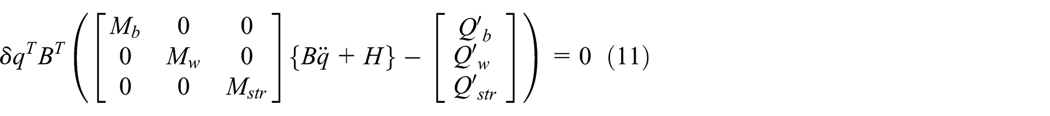
The variational form of the equations of motion is shown in equation (10)

$$\delta y{\prime }^T(M\stackrel{··}{y}\prime -Q)=0$$

(10)

where M is mass matrix. Q is the generalized force in each component of the body’s reference frame.

Using equations (9), equation (10) can be transformed to the generalized coordinate space

$$\delta q^T{B}^T(\left[\begin{array}{c}\hfill M_{b}00\hfill \\ \multicolumn{1}{c}{0M_{w}0}\\ \multicolumn{1}{c}{00M_{\mathrm{str}}}\end{array}\right]\{B\stackrel{··}{q}+H\}-\left[\begin{array}{c}\hfill {Q\prime }_b\hfill \\ \multicolumn{1}{c}{\begin{array}{c}\hfill {Q\prime }_w\hfill \\ \multicolumn{1}{c}{{Q\prime }_{\mathrm{str}}}\end{array}}\end{array}\right])=0$$

(11)

Since $\delta q$ is independent, equation (9) is valid for all $\delta q$ . Thus, the equation of motion for the vehicle model is

$$B^T\mathrm{MB}\stackrel{··}{q}=B^{T}Q-B^T\mathrm{MH}$$

(12)

where $B^T\mathrm{MB}$ is the mass matrix, $B^{T}Q$ is the applied force vector and $B^T\mathrm{MH}$ is a Coriolis and centrifugal force.

Suspension force model

A suspension system is installed between the chassis and wheel. Using the vectors that are associated with the body and wheels, the spring force and the damping force are defined using a spline function of the wheel travel $({\delta }_w)$ and vertical velocity $({\stackrel{·}{\delta }}_w)$ .

Tire force models

The quality of the vehicle dynamics model depends heavily on the tire model. The tire model used in this article is MF-Tire model, which is a semi-empirical mathematical model. ¹⁰ This model is a well-known tire model that is widely used in vehicle dynamic simulations. It calculates the forces (Fx, Fy) and moments (Mx, My, Mz) acting on the tire under pure and combined slip conditions on arbitrary roads. It uses longitudinal, lateral direction, turn slip, wheel inclination angle (‘camber’) and the vertical force (Fz) as input quantities.

In the model, the interaction forces and moments between the tire and the road surface are applied to a contact model. For these forces and moments to be calculated, the longitudinal velocity and lateral velocity of the contact point must be determined. This requires calculation of the longitudinal slip and slip angle. For a small slip condition, we can define the practical slip quantities $\alpha \prime$ and $\kappa \prime$ . The differential equation for these quantities can be written as the following equation (13)

$$\begin{array}{c}\multicolumn{1}{c}{{\sigma }_{\alpha }\frac{\mathrm{dv}}{\mathrm{dt}}+\left|{\stackrel{·}{x}}_r\right|v=-{\sigma }_{\alpha }{\stackrel{·}{y}}_{\mathrm{rs}}}\\ \multicolumn{1}{c}{{\sigma }_{\kappa }\frac{\mathrm{du}}{\mathrm{dt}}+\left|{\stackrel{·}{x}}_r\right|u=-{\sigma }_{\kappa }{\stackrel{·}{x}}_{\mathrm{rs}}}\end{array}$$

(13)

For the slip, the practical slip quantities $\alpha \prime$ and $\kappa \prime$ have been defined

$$\begin{array}{c}\multicolumn{1}{c}{\kappa \prime =\frac{u}{{\sigma }_k}\mathrm{sgn}\left({\stackrel{·}{x}}_r\right)}\\ \multicolumn{1}{c}{\alpha \prime =\mathrm{ta}{\mathrm{n}}^{-1}\left(\frac{v}{{\sigma }_{\alpha }}\right)}\end{array}$$

(14)

where ${\stackrel{·}{x}}_r$ , u, v, ${\sigma }_{\kappa }$ and ${\sigma }_{\alpha }$ are the tire velocity, longitudinal deflection, lateral deflection and tire relaxation lengths in the longitudinal and lateral directions, respectively. Using these practical slip quantities, the forces and moments can be calculated by fitting experimental data using the following equation

$$\begin{array}{c}\multicolumn{1}{c}{F=D_{\mathrm{MF}}\sin \left(C_{\mathrm{MF}}\arctan (B_{\mathrm{MF}}x-E_{\mathrm{MF}}(B_{\mathrm{MF}}x-\arctan \left(B_{\mathrm{MF}}x\right)))\right)+S_{\mathrm{MF}}}\\ \multicolumn{1}{c}{M=D_{\mathrm{MF}}\sin \left(C_{\mathrm{MF}}\arctan (B_{\mathrm{MF}}x-E_{\mathrm{MF}}(B_{\mathrm{MF}}x-\arctan \left(B_{\mathrm{MF}}x\right)))\right)+S_{\mathrm{MF}}}\end{array}$$

(15)

where F and M represent a tire force and moment, respectively. The variable x represents the input to which the tire slip ratio and angle respond. The coefficients $B_{\mathrm{MF}}$ , $C_{\mathrm{MF}}$ , $D_{\mathrm{MF}}$ and $E_{\mathrm{MF}}$ are factors that define the curve’s shape. $B_{\mathrm{MF}}$ is a stiffness factor, $C_{\mathrm{MF}}$ is a shape factor, $D_{\mathrm{MF}}$ is the peak value factor and $E_{\mathrm{MF}}$ is a curvature factor. ¹¹

Environment for simulation

The simulation algorithm was divided into four parts as shown in Figure 6. It begins using the initial condition such as vehicle properties, steering input, road profile and so on. Next, the model carries out the K&C analysis applying with the vehicle characteristics from K&C with respect to vehicle handling condition. And then, forces and torques acting on the body are calculated. Finally, the equations of motion are generated and solved using integration method.

Figure 6.

The flowchart for vehicle simulation.

Steering model

Steering model definition

A steering model is the additional dynamic model for the vehicle and the front tires which accounts for the delays in the steering system.^12,13 The steering actuation system consists of the actuator, shaft angle sensor and rotary spool valve (an integral part of the hydraulic power assist unit). Together with the rack and pinion, steering linkages and front wheels, the combined system can be approximated by a model with 4 DOF as shown in Figure 7. The actuator rotor inertia, upper shaft inertia, the pinion inertia, rack mass and steering linkage inertias are lumped into a single inertia. The wheel inertias are combined into a separate inertia.

Figure 7.

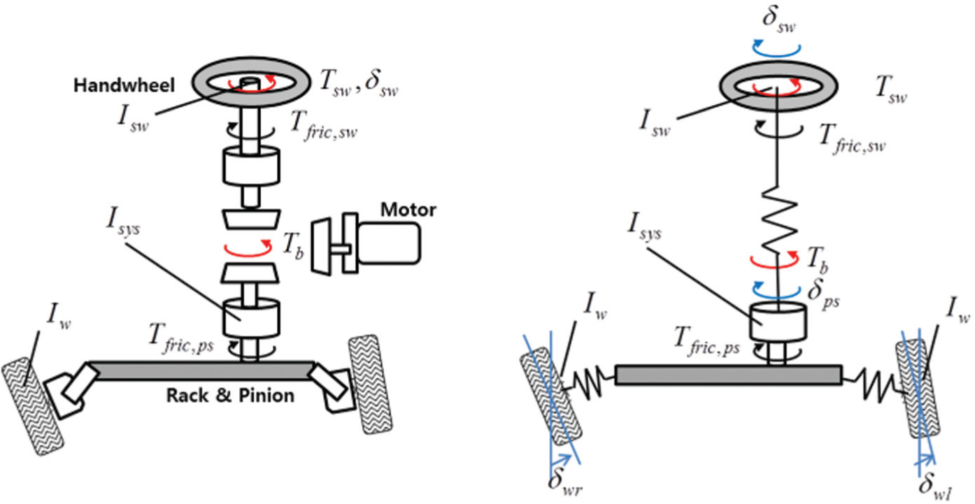
Steering model.

The equations of motion for this steering model are as follows

$$I_{\mathrm{sw}}{\stackrel{··}{\delta }}_{\mathrm{sw}}+C_{\mathrm{sw}}{\stackrel{·}{\delta }}_{\mathrm{sw}}+K_{\mathrm{sys}}({\delta }_{\mathrm{sw}}-{\delta }_{\mathrm{ps}})+T_{\mathrm{str}}=0$$

(16)

$$\begin{array}{c}\multicolumn{1}{c}{I_{\mathrm{sys}}{\stackrel{··}{\delta }}_{\mathrm{ps}}+C_{\mathrm{sys}}{\stackrel{·}{\delta }}_{\mathrm{ps}}+K_{\mathrm{sys}}({\delta }_{\mathrm{ps}}-{\delta }_{\mathrm{sw}})}\\ \multicolumn{1}{c}{+K_L(2\frac{{\delta }_{\mathrm{ps}}}{G_s}-{\delta }_{\mathrm{wl}}-{\delta }_{\mathrm{wr}})/G_s=T_b-T_{\mathrm{fric},\mathrm{ps}}}\end{array}$$

(17)

$$I_w{\stackrel{··}{\delta }}_{\mathrm{wr}}+C_w{\stackrel{·}{\delta }}_{\mathrm{wr}}+K_L({\delta }_{\mathrm{wr}}-\frac{{\delta }_{\mathrm{ps}}}{G_s})=-M{z}_{\mathrm{fr}}$$

(18)

$$I_w{\stackrel{··}{\delta }}_{\mathrm{wl}}+C_w{\stackrel{·}{\delta }}_{\mathrm{wl}}+K_L({\delta }_{\mathrm{wl}}-\frac{{\delta }_{\mathrm{ps}}}{G_s})=-M{z}_{\mathrm{fl}}$$

(19)

where ${\delta }_{\mathrm{sw}},{\delta }_{\mathrm{ps}},{\delta }_{\mathrm{wr}}$ and ${\delta }_{\mathrm{wl}}$ are the steering wheel angle, the column angle of steering system and wheel rotation angle of right and left side, respectively. $T_{\mathrm{str}},T_b$ and $T_{\mathrm{fric},\mathrm{ps}}$ are the torque applied on the steering wheel, motor and friction torque on pinion, respectively. $I_{\mathrm{sw}},I_{\mathrm{sys}}$ and $I_w$ are the moment of inertia of the steering wheel, lumped system and wheel, respectively. $K_{\mathrm{sys}}$ and $K_L$ are the stiffness of torsion bar and wheel linkage, respectively. $C_{\mathrm{sw}},C_{\mathrm{sys}}$ and $C_w$ are the viscous damping of steering wheel, column and linkage, respectively. $G_s$ is the steering gear ratio.

For the power steering system, the assist torque is defined as a function of torsion bar torque (T) and the vehicle speed by the following equation

$$f(T,{\stackrel{·}{x}}_b)=A_{\mathrm{motor}}·\tan \mathrm{h}(a\left({\stackrel{·}{x}}_b\right)·\cos \mathrm{h}(b\left({\stackrel{·}{x}}_b\right)·T)·\tan \mathrm{h}(c\left({\stackrel{·}{x}}_b\right)·T))$$

(20)

where $A_{\mathrm{motor}}$ is the maximum torque of motor. Variables a, b and c are the curve shape factor as a function of vehicle velocity. The friction torque is described by Dahl’s model ¹⁴

$${\stackrel{·}{T}}_{\mathrm{fric}}={\stackrel{·}{\delta }}_{\mathrm{ps}}{\gamma }_{\mathrm{fric}}{(T_{\mathrm{fric}}-f_{\mathrm{fric}}\mathrm{sign}\left({\stackrel{·}{\delta }}_{\mathrm{ps}}\right))}^2$$

(21)

where ${\gamma }_{\mathrm{fric}}$ and $f_{\mathrm{fric}}$ are the stiffness coefficient and Coulomb friction force, respectively.

Identification of steering model

Due to the lumped steering system model, the identification of parameters was conducted to achieve the best correlation result for steering stiffness. Figure 8 shows the process of identification. From the on-centre handling test, the objective value is calculated.

Figure 8.

The process for identification of steering system.

The objective function was to minimize the difference of steering stiffness value found between computation and the measurements. The steering stiffness is the slope which is taken using steering torque at minimum and maximum steering angle

$$\begin{array}{c}\multicolumn{1}{c}{\mathrm{minf}=|K_{\mathrm{str}}^{\mathrm{measure}}-K_{\mathrm{str}}^{\mathrm{sim}}|}\\ \multicolumn{1}{c}{K_{\mathrm{str}}=\frac{T_{\mathrm{str}}\left(\max \left({\delta }_{\mathrm{str}}\right)\right)-T_{\mathrm{str}}\left(\min \left({\delta }_{\mathrm{str}}\right)\right)}{\max \left({\delta }_{\mathrm{str}}\right)-\min \left({\delta }_{\mathrm{str}}\right)}}\end{array}$$

(22)

where $K_{\mathrm{str}}$ is the steering stiffness. Superscript ‘measure’ refers to obtaining data from a measurement, and ‘sim’ refers to the steering stiffness computed from the steering system model within the EVM simulation. To determine parameters $K_{\mathrm{sys}},K_L,C_{\mathrm{sw}},C_{\mathrm{sys}},C_w$ and ${\gamma }_{\mathrm{fric}},f_{\mathrm{fric}}$ of the lumped steering model, an evolutionary algorithm (EA) in PIAnO ¹⁵ was employed. An EA can be effective for solving difficult optimization problems, such as this one involving nonlinear global optimization. The target value was set from experimental data. The simulation was run with values for the coefficients. The difference between simulation and experimental data was compared. The algorithm was repeated until the solutions were within the accepted tolerance. After a successful optimization, values for the steering system parameters were obtained. The results are compared with the on-centre-handling test data in Figure 9. The steering stiffness behaviour is in good agreement between model and experiment.

Figure 9.

Identification of steering stiffness.

Full car test

The vehicle’s response to sudden step change steering input provides a reliable means to analyse the speed of response, vehicle stability under the existing conditions as well as the precision of the steering system. ¹⁶ In order to validate the vehicle simulation model, the step change steering test was performed with steering and gyro sensors installed on the chassis as shown in Figure 10(a). Beginning with straight driving at a constant speed of 60 km/h, the steering wheel is moved as fast as possible to the position that will result in a lateral acceleration of 4 m/s². The steering inputs were an amplitude of 55° and duration time of 0.2 s.

Figure 10.

Environment of test and the position of sensors: (a) position of sensors and (b) step change steering test.

Figures 11–13 compare the test results and EVM for reflecting rolling and steering characteristics about chassis lateral acceleration and yaw velocity. The EVM with all K&C characteristics has notably better agreement with the experimental data. And we compare with bicycle model and 14 DOF model which are not considering the K&C characteristics of vehicle.

Figure 11.

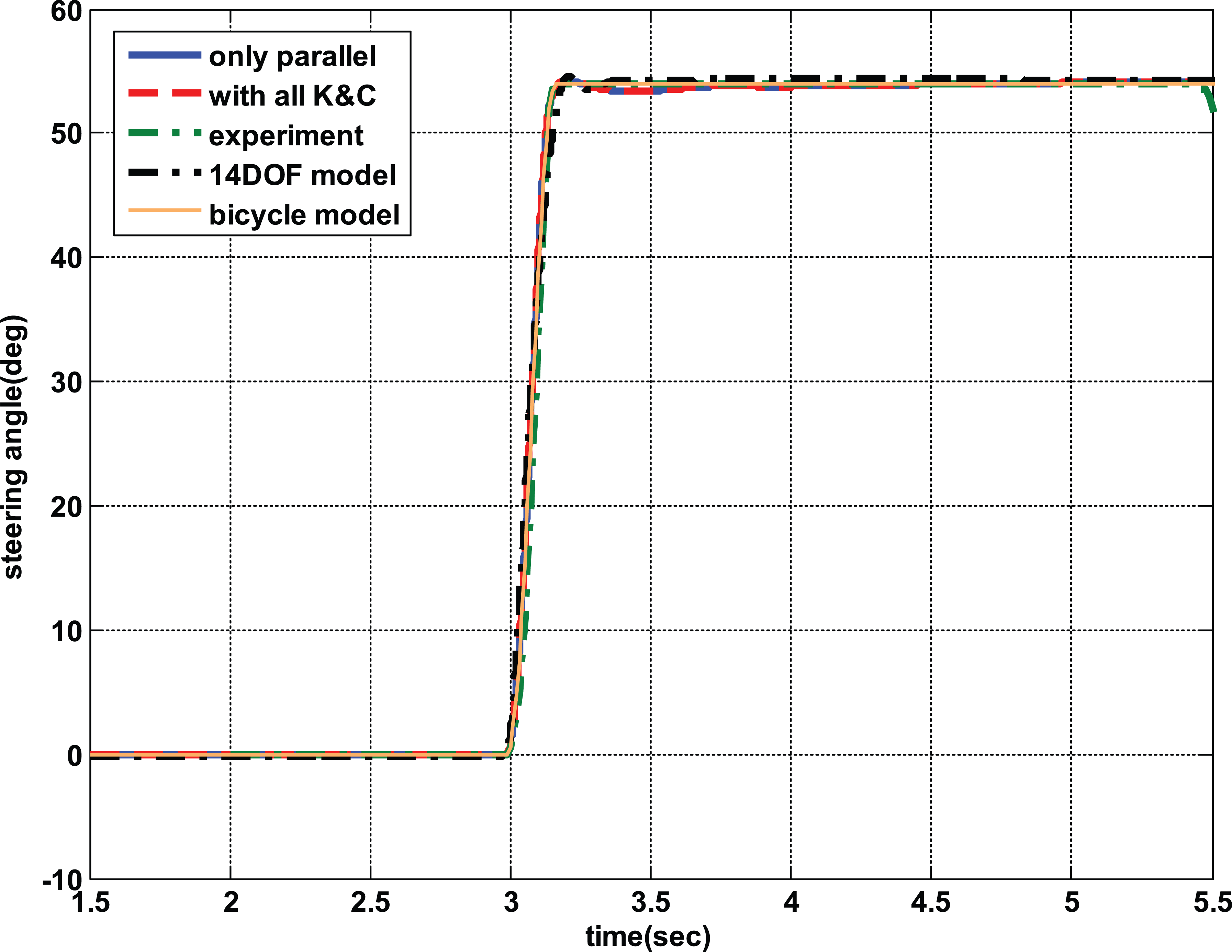
Comparison of steering angle.

Figure 12.

Comparison of body lateral acceleration.

Figure 13.

Comparison of body yaw rate.

The bicycle model is obviously different from experimental data because it does not include suspension roll effect. The 14-DOF model occurs at the overshoot, but at different responses. Most of all, Figures 11–13 show that two models need the K&C characteristics to reduce the difference. The movement of the wheel travel and steering angle affects the lateral and yaw moments acting on the sprung mass. This movement also affects the load transfer. In extreme manoeuvres, these phenomena can significantly affect the vehicle handling response. A vehicle model that includes all K&C characteristics will be needed to model these effects.

To compare the accuracy of this article, EVM in this article was compared to FVM in Yuen et al. ⁸ Since EVM in this article was a more precise model than the FVM, the result showed more accurate than the FVM. As shown in Table 1, the error on step steer test was reduced with the EVM, in which yaw rate overshoot was much decreased in EVM. The FVM just employed an opposite test result and the toe angle with respect to body roll motion. In the EVM, K&C information such as caster, camber, toe, wheel tread and wheelbase measured from SPMD seemed to enhance the accuracy.

Table 1.

Comparison of error between FVM and EVM.

	Result with FVM (Yuen et al.’s paper 8 )	Result with EVM (this article)
Steady-state lateral acc. (%)	4.76	2.39
Overshoot of lateral acc. (%)	9.21	2.95
Steady-state yaw rate (%)	4.40	3.32
Overshoot of yaw rate (%)	20.14	2.22
Steady-state roll angle (%)	3.54	3.02
Overshoot of roll angle (%)	2.91	2.19

FVM: full vehicle model; EVM: experimental vehicle model; acc.: acceleration.

Conclusion

The main objective of this study was to derive a dynamic vehicle model which incorporates K&C test results. The steering model has been modelled with a 4-DOF lumped model and identified system parameters from the experiment data using PIAnO. For the verification of the model, the simulation result was validated by comparing it with a full vehicle test:

1. The research was able to incorporate experimental K&C data from SPMD. Tire and steering system performance was also incorporated using experimental data.

2. The lumped steering model is recommended. Using experimental data, the system physical parameters were identified.

3. Comparing the step change steering simulation and experiment, the model with all K&C data was validated. It also showed the quality improvement of handling performance.

It is expected that these results can be applied to additional vehicle models and contribute to additional improvements in automotive handling qualities.