Numerical solution for the model of RLC circuit via the fractional derivative without singular kernel

Abstract

The numerical approximation of the Caputo–Fabrizio fractional derivative with fractional order between 1 and 2 is proposed in this work. Using the transition from ordinary derivative to fractional derivative, we modified the RLC circuit model. The Crank–Nicolson numerical scheme was used to solve the modified model. We present the stability analysis of the numerical scheme for solving the modified equation and some numerical simulations for different values of the order of derivation.

Introduction

In the recent decade, several researchers have proposed new definitions of the concept of derivative with fractional order. These definitions go from Riemann–Liouville to the newly proposed one by Caputo and Fabrizio. The old editions of the designed definition of the fractional derivative are a product of convolution of a derivative of a function $f(x)$ with the function $x^{1-\alpha }$ in the case of Caputo old edition, and $f(x)$ and the function $x^{1-\alpha }$ in the case of Riemann–Liouville.^1–6 Both the Riemann–Liouville and Caputo old version are designed with singular kernel. Several researchers have used the derivatives across all fields of sciences and engineering for modeling real-world problems. Recently, a new mathematical design of the concept of derivative with fractional was proposed by Caputo and Fabrizio.^7–9 The proposed derivative with fractional order is the convolution of first derivative and the function exponential; with this definition, there is no worry of singular kernel, and therefore, any model using this new derivative describes the full effect of the memory for the problem. The new Caputo–Fabrizio derivative is presented in the following definition.

Definition 1. Let $f(x)$ be continuous and differentiable on $C^1[0,1]$ , then the Caputo–Fabrizio derivate with fractional order $0<\alpha \le 1$ is given as follows

$${{}_0{}^{CF}D}_x^{\alpha }f\left(x\right)=\frac{M\left(\alpha \right)}{1-\alpha }\underset{0}{\overset{x}{\int }}\frac{\text{d}f\left(t\right)}{\text{d}t}\exp [-\alpha \frac{x-t}{1-\alpha }]\mathrm{dt}$$

(1)

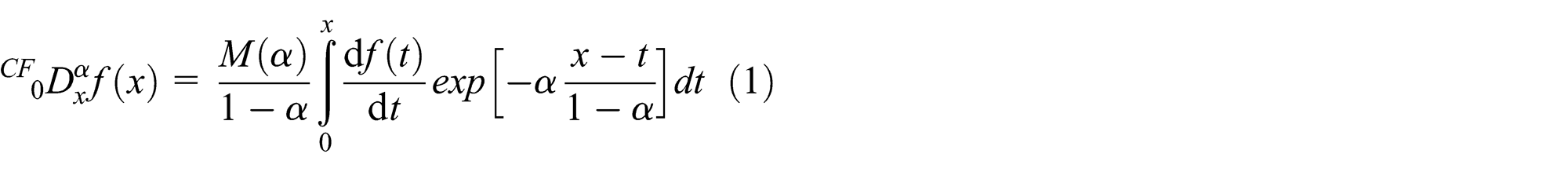
In the above definition, the function M is a normalized function that takes the value 1 when α takes the values 0 and 1.^7–9 The anti-derivative associated with the new derivative was proposed by Losada and Nieto and is given as follows.

Definition 2. Let $0<\alpha <1$ . The fractional integral of Caputo–Fabrizio type must be defined as follows

$${{}_0{}^{CF}I}_t^{\alpha }f\left(t\right)=\frac{2(1-\alpha )}{(2-\alpha )M\left(\alpha \right)}f\left(t\right)+\frac{2\alpha }{(2-\alpha )M\left(\alpha \right)}\underset{0}{\overset{t}{\int }}f\left(x\right)\mathrm{dx}$$

(2)

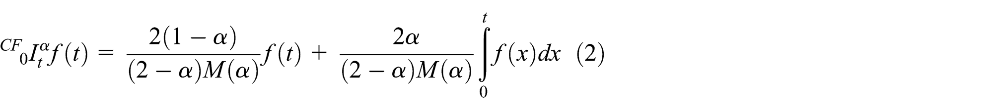
Losada and Nieto remarked that according to Definition 2, the fractional integral of Caputo-type of a function of order $0<\alpha <1$ is an average between function and its integral of order 1.^7–9 Their remark imposed that

$$\frac{2(1-\alpha )}{(2-\alpha )M\left(\alpha \right)}+\frac{2\alpha }{(2-\alpha )M\left(\alpha \right)}=1$$

(3)

The above condition allowed them to find a particular case of the normalized function

$$M\left(\alpha \right)=\frac{2}{2-\alpha },0<\alpha <1$$

Without any doubt, this new derivative will be used in all the branches of sciences for modeling. ⁸ In order to translate from ordinary differential equations to fractional differential equations, we present the following mathematical transition for the time and space components: for the time component, we have

$$\begin{array}{cc}\multicolumn{1}{c}{}& \frac{\text{d}}{\text{d}t}\to \frac{1}{\exp [-\frac{(1-\alpha ){\sigma }_t}{2-\alpha }]}{{}_0{}^{CF}D}_t^{\alpha },\hfill \\ \multicolumn{1}{c}{}& \frac{\text{d}}{\text{d}x}\to \frac{1}{\exp [-\frac{(1-\alpha ){\sigma }_x}{2-\alpha }]}{{}_0{}^{CF}D}_x^{\alpha }\hfill \end{array}$$

(4)

The new parameters ${\sigma }_t$ and ${\sigma }_x$ are called time and space scale parameters. These new parameters have the dimension of length (m) and time (s); they characterize the fractional space and fractional temporal structures, in particular components that show an intermediate behavior between a system conservative and dissipative. ⁹ Note that when α is 1, we recover the ordinary derivative of order 1. The aim of this article is to further access the efficiency of the newly proposed derivative with fractional order by applying it to the model of transmission line with losses and solves the resulting equation numerically. The model under investigation here is given as follows

$$\begin{array}{cc}\multicolumn{1}{c}{}& \frac{{\partial }^{2}V(x,t)}{\partial x^2}-\frac{\mathrm{LC}{\partial }^{2}V(x,t)}{\partial t^2}-(\mathrm{RC}+\mathrm{GL})\hfill \\ \multicolumn{1}{c}{}& \frac{\partial V(x,t)}{\partial t}-\mathrm{GRV}(x,t)=0\hfill \end{array}$$

(5)

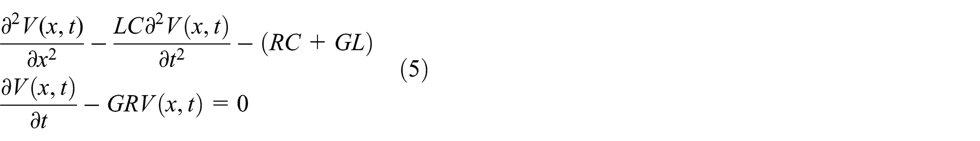
In the above equation, L is the representation of the inductance because of the magnetic field around the wires, C is the capacitance between the two conductors, R is the resistance of the conductors, and G is the conductance of the electric material separating the conductors. ¹⁰

Using the proposed transition, we suggest the following fractional RLC circuit model

$$\begin{array}{cc}\multicolumn{1}{c}{}& \frac{1}{\exp [-\frac{\beta {\sigma }_x}{2-\beta }]}{{}_0{}^{CF}D}_x^{\beta }(V(x,t))-\frac{\mathrm{LC}}{\exp [-\frac{\beta {\sigma }_t}{2-\beta }]}{{}_0{}^{CF}D}_x^{\beta }\left(V(x,t)\right)\hfill \\ \multicolumn{1}{c}{}& -\frac{(\mathrm{RC}+\mathrm{GL})}{\exp [-\frac{(1-\alpha ){\sigma }_t}{2-\alpha }]}\left\{{{}_0{}^{CF}D}_t^{\alpha }(V(x,t))\right\}-\mathrm{GRV}(x,t)=0\hfill \end{array}$$

with $1<\beta <2;0<\alpha <1$

We shall present in the next section the numerical approximation of space and time Caputo–Fabrizio derivative with fractional order.

Numerical approximation of the new fractional derivative

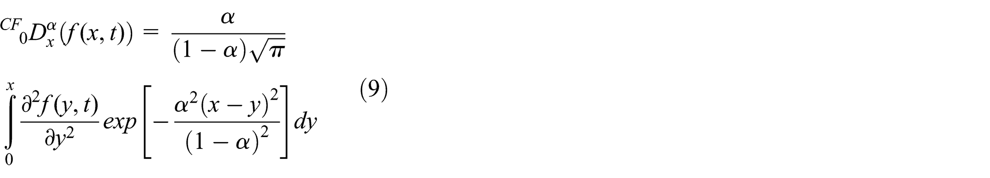
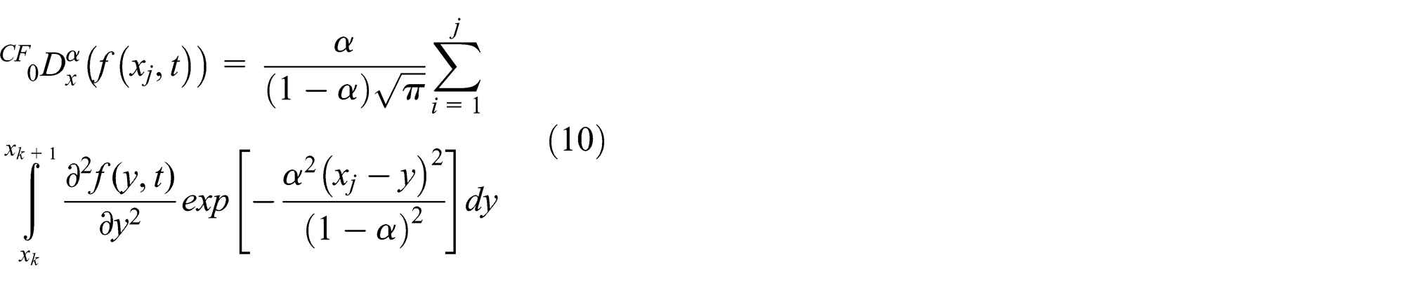
Definition 3.

1. Let $f(t)$ be a function in $C^2[a,b]$ and let the order of the fractional derivative be $0<\alpha \le 1$ , then the first-order approximation of the Caputo–Fabrizio derivative at a point $t_n$ is

   $$\begin{array}{cc}\multicolumn{1}{c}{{{}_0{}^{CF}D}_t^{\alpha }\left(f\left(t_n\right)\right)=}& \frac{M\left(\alpha \right)}{\alpha }\sum _{j=1}^n\left(\frac{f^{j+1}-f^j}{k}\right)d_{j,k}\hfill \\ \multicolumn{1}{c}{}& +\frac{M\left(\alpha \right)}{\alpha }\sum _{j=1}^n{d}_{j,k}O\left(k\right)\hfill \end{array}$$

   (6)

   where

   $$\begin{array}{cc}\multicolumn{1}{c}{d_{j,k}=}& -\exp [-\alpha \frac{k}{1-\alpha }(n-j+1)]\hfill \\ \multicolumn{1}{c}{}& +\exp [-\alpha \frac{k}{1-\alpha }(n-j)]\hfill \end{array}$$

2. Let $f(x,t)$ be a function in $C^2([a,b]\times [0,T])$ and let the order of the fractional derivative be $0<\alpha \le 1$ , then the first-order approximation of the Caputo–Fabrizio derivative at a point $(x_m,t_n)$ is

   $$\begin{array}{cc}\multicolumn{1}{c}{}& {{}_0{}^{CF}D}_x^{\alpha }\left(f(x_m,t_k)\right)=\frac{M\left(\alpha \right)}{1-\alpha }\sum _{l=1}^m\hfill \\ \multicolumn{1}{c}{}& \{\frac{(f_{i+1}^{k+1}-f_{i-1}^{k+1})-(f_{i+1}^k-f_{i-1}^k)}{4i}\frac{(1-\alpha )\sqrt{\pi }}{2\alpha }\hfill \\ \multicolumn{1}{c}{}& \{\mathrm{erf}\left[(m-l)\frac{\alpha i}{1-\alpha }\right]-\mathrm{erf}\left[(m-l+1)\frac{\alpha i}{1-\alpha }\right]\}\}\hfill \\ \multicolumn{1}{c}{}& +O\left(i\right)\frac{(1-\alpha )}{2\alpha }\sum _{l=1}^m\hfill \\ \multicolumn{1}{c}{}& \{\mathrm{erf}\left[(m-l)\frac{\alpha i}{1-\alpha }\right]-\mathrm{erf}\left[(m-l+1)\frac{\alpha i}{1-\alpha }\right]\}\hfill \end{array}$$

   (7)

Theorem 1. Let $f(x,t)$ be twice differentiable on both $x$ and $t$ directions, then the second derivative approximation of the Caputo–Fabrizio derivative of $f(x,t)$ is given as

$$\begin{array}{cc}\multicolumn{1}{c}{}& {{}_0{}^{CF}D}_x^{\alpha }\left(f(x_j,t)\right)=\frac{1}{2}\sum _{k=1}^j\hfill \\ \multicolumn{1}{c}{}& \left\{\frac{(f_{i+1}^{k+1}-2f_i^{k+1}+f_{i-1}^{k+1})+(f_{i+1}^k-2f_i^k+f_{i-1}^k)}{2{\left(\Delta x\right)}^2}\right\}\hfill \\ \multicolumn{1}{c}{}& \{\mathrm{erf}\left[\frac{\alpha }{1-\alpha }(x_j-x_{k+1})\right]-\mathrm{erf}\left[\frac{\alpha }{1-\alpha }(x_j-x_k)\right]\}\hfill \\ \multicolumn{1}{c}{}& +O\left({(\Delta x)}^2\right)\hfill & \hfill \end{array}$$

(8)

Proof. The corresponding second order of the new fractional derivative is given by

$$\begin{array}{cc}\multicolumn{1}{c}{}& {{}_0{}^{CF}D}_x^{\alpha }(f(x,t))=\frac{\alpha }{(1-\alpha )\sqrt{\pi }}\hfill \\ \multicolumn{1}{c}{}& \underset{0}{\overset{x}{\int }}\frac{{\partial }^{2}f(y,t)}{\partial y^2}\exp [-\frac{{\alpha }^2{(x-y)}^2}{{(1-\alpha )}^2}]\mathrm{dy}\hfill \end{array}$$

(9)

However, for any given $x_j$ , we have

$$\begin{array}{cc}\multicolumn{1}{c}{}& {{}_0{}^{CF}D}_x^{\alpha }\left(f(x_j,t)\right)=\frac{\alpha }{(1-\alpha )\sqrt{\pi }}\sum _{i=1}^j\hfill \\ \multicolumn{1}{c}{}& \underset{x_k}{\overset{x_{k+1}}{\int }}\frac{{\partial }^{2}f(y,t)}{\partial y^2}\exp [-\frac{{\alpha }^2{(x_j-y)}^2}{{(1-\alpha )}^2}]\mathrm{dy}\hfill \end{array}$$

(10)

Using the Crank–Nicolson scheme for the usual second-order derivative, the above equation can be reformulated as

$$\begin{array}{cc}\multicolumn{1}{c}{}& {{}_0{}^{CF}D}_x^{\alpha }\left(f(x_j,t)\right)=\frac{\alpha }{(1-\alpha )\sqrt{\pi }}\sum _{i=1}^j\hfill \\ \multicolumn{1}{c}{}& \{\frac{(f_{i+1}^{k+1}-2f_i^{k+1}+f_{i-1}^{k+1})+(f_{i+1}^k-2f_i^k+f_{i-1}^k)}{2{\left(\Delta x\right)}^2}+O\left({(\Delta x)}^2\right)\}\hfill \\ \multicolumn{1}{c}{}& \left[\underset{x_k}{\overset{x_{k+1}}{\int }}\exp [-\frac{{\alpha }^2{(x_j-y)}^2}{{(1-\alpha )}^2}]\mathrm{dy}\right],f(x_j,t_i)=f_i^j\hfill \end{array}$$

(11)

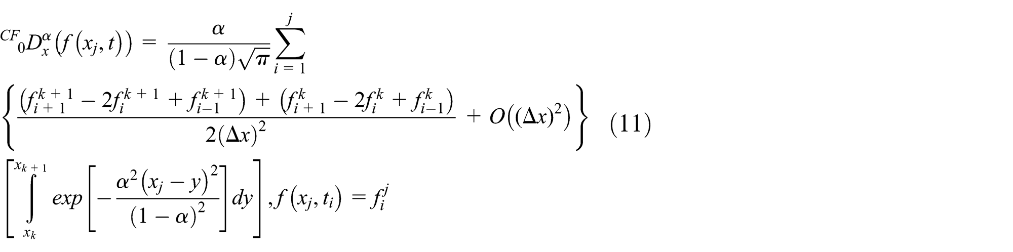
Nevertheless, the integral in the right-hand side is evaluated as

$$\begin{array}{cc}\multicolumn{1}{c}{}& \underset{x_k}{\overset{x_{k+1}}{\int }}\exp [-\frac{{\alpha }^2{(x_j-y)}^2}{{(1-\alpha )}^2}]\mathrm{dy}=\frac{(1-\alpha )\sqrt{\pi }}{2\alpha }\hfill \\ \multicolumn{1}{c}{}& \{\mathrm{erf}\left[\frac{\alpha }{1-\alpha }(x_j-x_{k+1})\right]-\mathrm{erf}\left[\frac{\alpha }{1-\alpha }(x_j-x_k)\right]\}\hfill \end{array}$$

(12)

Therefore, equation (11) becomes

$$\begin{array}{cc}\multicolumn{1}{c}{}& {{}_0{}^{CF}D}_x^{\alpha }\left(f(x_j,t)\right)=\frac{1}{2}\sum _{i=1}^j\hfill \\ \multicolumn{1}{c}{}& \{\frac{(f_{i+1}^{k+1}-2f_i^{k+1}+f_{i-1}^{k+1})+(f_{i+1}^k-2f_i^k+f_{i-1}^k)}{2{\left(\Delta x\right)}^2}+O\left({(\Delta x)}^2\right)\}\hfill \\ \multicolumn{1}{c}{}& \{\mathrm{erf}\left[\frac{\alpha }{1-\alpha }(x_j-x_{k+1})\right]-\mathrm{erf}\left[\frac{\alpha }{1-\alpha }(x_j-x_k)\right]\}\hfill \end{array}$$

(13)

The above equation can be rewritten as follows

$$\begin{array}{cc}\multicolumn{1}{c}{}& {{}_0{}^{CF}D}_x^{\alpha }\left(f(x_j,t)\right)=\frac{1}{2}\sum _{i=1}^j\hfill \\ \multicolumn{1}{c}{}& \left\{\frac{(f_{i+1}^{k+1}-2f_i^{k+1}+f_{i-1}^{k+1})+(f_{i+1}^k-2f_i^k+f_{i-1}^k)}{2{\left(\Delta x\right)}^2}\right\}\hfill \\ \multicolumn{1}{c}{}& \{\mathrm{erf}\left[\frac{\alpha }{1-\alpha }(x_j-x_{k+1})\right]-\mathrm{erf}\left[\frac{\alpha }{1-\alpha }(x_j-x_k)\right]\}\hfill \\ \multicolumn{1}{c}{}& +\sum _{i=1}^j\{\mathrm{erf}\left[\frac{\alpha }{1-\alpha }(x_j-x_{k+1})\right]-\mathrm{erf}\left[\frac{\alpha }{1-\alpha }(x_j-x_k)\right]\}\hfill \\ \multicolumn{1}{c}{}& O\left({\left(\Delta x\right)}^2\right)\hfill & \hfill \end{array}$$

(14)

Note that

$$\begin{array}{cc}\multicolumn{1}{c}{}& \sum _{k=1}^j\{\mathrm{erf}\left[\frac{\alpha }{1-\alpha }(x_j-x_{k+1})\right]-\mathrm{erf}\left[\frac{\alpha }{1-\alpha }(x_j-x_k)\right]\}\hfill \\ \multicolumn{1}{c}{}& =\mathrm{erf}\left[\frac{-j\alpha }{1-\alpha }\Delta x\right]\hfill \end{array}$$

(15)

Using the Abromowitz and Stegun series approximation of the error function, equation (14) is reduced to

$$\begin{array}{cc}\multicolumn{1}{c}{}& {{}_0{}^{CF}D}_x^{\alpha }\left(f(x_j,t)\right)=\frac{1}{2}\sum _{i=1}^j\hfill \\ \multicolumn{1}{c}{}& \left\{\frac{(f_{i+1}^{k+1}-2f_i^{k+1}+f_{i-1}^{k+1})+(f_{i+1}^k-2f_i^k+f_{i-1}^k)}{2{\left(\Delta x\right)}^2}\right\}\hfill \\ \multicolumn{1}{c}{}& \{\mathrm{erf}\left[\frac{\alpha }{1-\alpha }(x_j-x_{k+1})\right]-\mathrm{erf}\left[\frac{\alpha }{1-\alpha }(x_j-x_k)\right]\}\hfill \\ \multicolumn{1}{c}{}& +O\left({\left(\Delta x\right)}^2\right)\hfill & \hfill \end{array}$$

(16)

This completes the proof.

Numerical solution of time fractional transmission line with losses

For some positive integer N, the grid sizes in time for finite difference technique I are defined by

$$k=\frac{1}{N}$$

The grid points in the time interval $[0,T]$ are labeled $t_n=\mathrm{nk},n=0,1,2,\dots ,\mathrm{TN}$

For some positive integer N, the grid sizes in time for finite difference technique I are defined by

$$i=\frac{1}{M}$$

The grid points in the time interval $[0,X]$ are labeled $x_i=\mathrm{mi},m=0,1,2,\dots ,\mathrm{XM}$ . The modified model of transmission line with losses is

$$\begin{array}{cc}\multicolumn{1}{c}{}& \frac{1}{\exp [-\frac{\beta {\sigma }_x}{2-\beta }]}{{}_0{}^{CF}D}_x^{\beta }(V(x,t))\hfill \\ \multicolumn{1}{c}{}& -\frac{\mathrm{LC}}{\exp [-\frac{\beta {\sigma }_t}{2-\beta }]}{{}_0{}^{CF}D}_x^{\beta }\left(V(x,t)\right)\hfill \\ \multicolumn{1}{c}{}& -\frac{(\mathrm{RC}+\mathrm{GL})}{\exp [-\frac{(1-\alpha ){\sigma }_t}{2-\alpha }]}\left\{{{}_0{}^{CF}D}_t^{\alpha }\left(V(x,t)\right)\right\}-\mathrm{GRV}(x,t)\hfill \\ \multicolumn{1}{c}{}& =0,1<\beta <2;0<\alpha <1\hfill \end{array}$$

(17)

with initial and boundary conditions

$$V(x,0)=f\left(x\right),V(0,t)=g\left(t\right)$$

The main aim of this section is to solve the above equation numerically using the well-known Crank–Nicolson numerical scheme. To achieve this, we first replace in equation (17) the numerical approximation of space and time fractional Caputo–Fabrizio derivative, and this produces

$$\begin{array}{cc}\multicolumn{1}{c}{}& \frac{1}{\exp [-\frac{\beta {\sigma }_x}{1-\beta }]}\left\{\frac{1}{2}\sum _{i=1}^m\left\{\frac{(V_{i+1}^{k+1}-2V_i^{k+1}+V_{i-1}^{k+1})+(V_{i+1}^k-2V_i^k+V_{i-1}^k)}{2{\left(\Delta x\right)}^2}\right\}\{\mathrm{erf}\left[\frac{\beta }{1-\beta }(x_j-x_{k+1})\right]-\mathrm{erf}\left[\frac{\beta }{1-\beta }(x_j-x_k)\right]\}\right\}\hfill \\ \multicolumn{1}{c}{}& -\frac{\mathrm{LC}}{\exp [-\frac{\beta {\sigma }_t}{2-\beta }]}\left\{\frac{1}{2}\sum _{k=1}^j\left\{\frac{(V_{i+1}^{k+1}-2V_i^{k+1}+V_{i-1}^{k+1})}{2{\left(\Delta t\right)}^2}\right\}\{\mathrm{erf}[-\frac{\beta k}{1-\beta }(n-j+1)]-\mathrm{erf}[-\frac{\beta k}{1-\beta }(n-j)]\}\right\}\hfill \\ \multicolumn{1}{c}{}& -\frac{(\mathrm{RC}+\mathrm{GL})}{\exp [-\frac{\left(\alpha \right){\sigma }_t}{1-\alpha }]}\{\frac{M\left(\alpha \right)}{\alpha }\sum _{k=1}^j\left(\frac{V_i^{k+1}-V_i^k}{\Delta t}\right)\exp [-\alpha \frac{k}{1-\alpha }(n-j+1)]-\exp [-\alpha \frac{k}{1-\alpha }(n-j)]\}-\mathrm{GR}\left(\frac{V_i^{j+1}-V_i^j}{2}\right)=0\hfill \end{array}$$

(18)

For simplicity, let us put

$$\begin{array}{cc}\multicolumn{1}{c}{g_{n,j,k}=}& \exp [-\alpha \frac{k}{1-\alpha }(n-j+1)]\hfill \\ \multicolumn{1}{c}{}& -\exp [-\alpha \frac{k}{1-\alpha }(n-j)]\hfill \end{array}$$

$$d_{n,j,k}=\{\mathrm{erf}\left[\frac{\alpha }{1-\alpha }(x_j-x_{k+1})\right]-\mathrm{erf}\left[\frac{\alpha }{1-\alpha }(x_j-x_k)\right]\}$$

$$\begin{array}{cc}\multicolumn{1}{c}{}& p_{\alpha }=\frac{(\mathrm{RC}+\mathrm{GL})}{2(\Delta t)\exp [-\frac{(\alpha ){\sigma }_t}{1-\alpha }]}\frac{M\left(\alpha \right)}{\alpha },\hfill \\ \multicolumn{1}{c}{}& v_{\alpha }=\frac{\mathrm{LC}}{2{\left(\Delta t\right)}^2\exp [-\frac{\beta {\sigma }_t}{2-\beta }]},\hfill \\ \multicolumn{1}{c}{}& b_{\beta }=\frac{1}{2{\left(\Delta x\right)}^2\exp [-\frac{\beta {\sigma }_x}{1-\beta }]}\hfill \end{array}$$

Stability analysis

In this section, we will use the Fourier method to establish the stability of the numerical method used to solve the modified time fractional transmission line with losses model. Equation (18) can now become

$$\begin{array}{cc}\multicolumn{1}{c}{}& b_{\beta }\left\{\frac{1}{2}\sum _{l=1}^i\{(V_{l+1}^{j+1}-2V_l^{j+1}+V_{l-1}^{j+1})+(V_{l+1}^j-2V_l^j+V_{l-1}^j)\}{d}_{i,j,l}\right\}\hfill \\ \multicolumn{1}{c}{}& -v_{\alpha }\left\{\frac{1}{2}\sum _{k=1}^j\{V_{i+1}^{k+1}-2V_i^{k+1}+V_{i-1}^{k+1}\}{d}_{n,j,k}\right\}\hfill \\ \multicolumn{1}{c}{}& -p_{\alpha }\left\{\sum _{k=1}^j(V_i^{k+1}-V_i^k)g_{n,j,k}\right\}-\mathrm{GR}\left(\frac{V_i^{j+1}-V_i^j}{2}\right)=0\hfill \end{array}$$

(19)

We let $v_i^j-V_i^j={\beta }_i^j$ with $V_i^j$ the approximate solution at the point $(x_i,t_j)$ and commonly ${\beta }^j=[{\beta }_1^j,\dots ,{\beta }_N^j{]}^{\text{T}}$ . The analysis of stability of the used scheme can be achieved if we assume that

$${\beta }_i^j=h\left(j\right)e^{m_x{x}_i}$$

(20)

By replacing the above equation (20) into equation (19) and, for simplicity, assuming that β is 1, equation (1) becomes

$$\begin{array}{cc}\multicolumn{1}{c}{}& h(j+1)(8\mathrm{si}{n}^2\left(\frac{m_x{x}_i}{2}\right)b_1+v_{\alpha }{d}_{n,j,j}+p_{\alpha }{g}_{n,j,j}+2\mathrm{si}{n}^2\left(\frac{m_x{x}_i}{2}\right)\mathrm{GR})\hfill \\ \multicolumn{1}{c}{}& =h\left(j\right)(-8\mathrm{si}{n}^2\left(\frac{m_x{x}_i}{2}\right)b_1+p_{\alpha }{g}_{n,j,j}+2\mathrm{si}{n}^2\left(\frac{m_x{x}_i}{2}\right)\mathrm{GR})\hfill \\ \multicolumn{1}{c}{}& +\sum _{k=1}^{j-1}(g_{n,j,k}{p}_{\alpha }-v_{\alpha }{d}_{n,j,k})h(k+1)-p_{\alpha }\sum _{k=1}^{j-1}h(k)g_{n,j,k}\hfill \end{array}$$

(21)

If $1<j$ , the part with summation produces zero; therefore, $0=j$ , and equation (21) becomes

$$\begin{array}{cc}\multicolumn{1}{c}{h\left(1\right)}& (8\mathrm{si}{n}^2\left(\frac{m_x{x}_i}{2}\right)b_1+v_{\alpha }{d}_{n,j,j}+p_{\alpha }{g}_{n,j,j}\hfill \\ \multicolumn{1}{c}{}& +2\mathrm{si}{n}^2\left(\frac{m_x{x}_i}{2}\right)\mathrm{GR})=h\left(0\right)\hfill \\ \multicolumn{1}{c}{}& (-8\mathrm{si}{n}^2\left(\frac{m_x{x}_i}{2}\right)b_1+p_{\alpha }{g}_{n,j,j}+2\mathrm{si}{n}^2\left(\frac{m_x{x}_i}{2}\right)\mathrm{GR})\hfill \end{array}$$

(22)

Then, rearranging and applying on both sides the absolute value, we obtain

$$\begin{array}{cc}\multicolumn{1}{c}{}& \left|\frac{h\left(1\right)}{h\left(0\right)}\right|=\hfill \\ \multicolumn{1}{c}{}& \left|\frac{(-8\mathrm{si}{n}^2\left(\frac{m_x{x}_i}{2}\right)b_1+p_{\alpha }{g}_{n,j,j}+2\mathrm{si}{n}^2\left(\frac{m_x{x}_i}{2}\right)\mathrm{GR})}{(8\mathrm{si}{n}^2\left(\frac{m_x{x}_i}{2}\right)b_1+v_{\alpha }{d}_{n,j,j}+p_{\alpha }{g}_{n,j,j}+2\mathrm{si}{n}^2\left(\frac{m_x{x}_i}{2}\right)\mathrm{GR})}\right|<1\hfill \end{array}$$

(23)

This implies

$$\left|\frac{h\left(1\right)}{h\left(0\right)}\right|<1$$

Theorem 2. Assuming that $h(j)$ is the solution of equation (21), then, for every integer number $j$ greater or equal to 1, the following relation is satisfied

$$h\left(j\right)<h\left(0\right)$$

(24)

Proof. We achieve this proof by employing the recursive technique on the natural number $j$ . The proof is verified for $j=0$ , see above. Now we assume that for any k greater than 1, the inequality is satisfied, then, for $k=j$ , and we have the following

$$\begin{array}{cc}\multicolumn{1}{c}{}& h\left(j\right)(-8\mathrm{si}{n}^2\left(\frac{m_x{x}_i}{2}\right)b_1+v_{\alpha }{d}_{n,j,j}+p_{\alpha }{g}_{n,j,j}+2\mathrm{si}{n}^2\left(\frac{m_x{x}_i}{2}\right)\mathrm{GR})\hfill \\ \multicolumn{1}{c}{}& =h(j-1)(8\mathrm{si}{n}^2\left(\frac{m_x{x}_i}{2}\right)b_1+p_{\alpha }{g}_{n,j,j}+2\mathrm{si}{n}^2\left(\frac{m_x{x}_i}{2}\right)\mathrm{GR})\hfill \\ \multicolumn{1}{c}{}& +\sum _{k=1}^{j-1}(g_{n,j,k}{p}_{\alpha }-v_{\alpha }{d}_{n,j,k})h(k+1)-p_{\alpha }\sum _{k=1}^{j-1}h\left(k\right)g_{n,j,k}\hfill \end{array}$$

(25)

Therefore, applying the norm on both sides, we obtain the following result

$$\begin{array}{cc}\multicolumn{1}{c}{}& \Vert h\left(j\right)(8\mathrm{si}{n}^2\left(\frac{m_x{x}_i}{2}\right)b_1+v_{\alpha }{d}_{n,j,j}+p_{\alpha }{g}_{n,j,j}+2\mathrm{si}{n}^2\left(\frac{m_x{x}_i}{2}\right)\mathrm{GR})\Vert \hfill \\ \multicolumn{1}{c}{}& \le \Vert h(j-1)(-8\mathrm{si}{n}^2\left(\frac{m_x{x}_i}{2}\right)b_1+p_{\alpha }{g}_{n,j,j}+2\mathrm{si}{n}^2\left(\frac{m_x{x}_i}{2}\right)\mathrm{GR})\Vert \hfill \\ \multicolumn{1}{c}{}& \Vert \sum _{k=1}^{j-1}(g_{n,j,k}{p}_{\alpha }-v_{\alpha }{d}_{n,j,k})h(k+1)-p_{\alpha }\sum _{k=1}^{j-1}h(k)g_{n,j,k}\Vert \hfill \end{array}$$

(26)

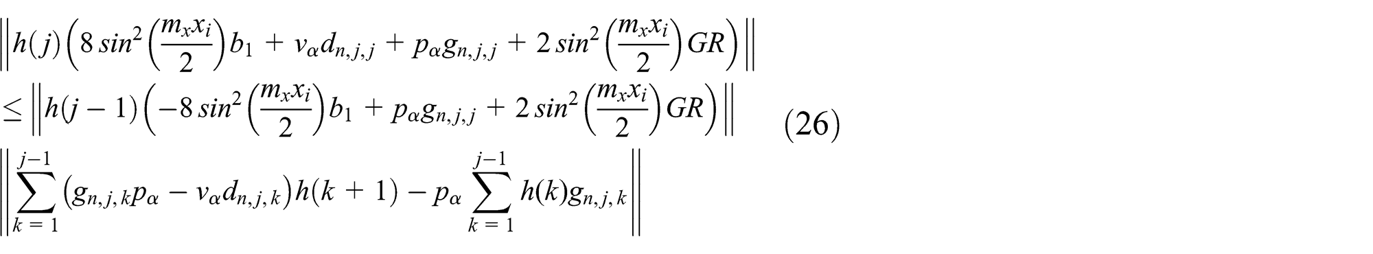
Employing the triangular equality and other properties, we obtain

$$\begin{array}{cc}\multicolumn{1}{c}{}& \Vert h\left(j\right)\Vert \left|(8\mathrm{si}{n}^2\left(\frac{m_x{x}_i}{2}\right)b_1+v_{\alpha }{d}_{n,j,j}+p_{\alpha }{g}_{n,j,j}+2\mathrm{si}{n}^2\left(\frac{m_x{x}_i}{2}\right)\mathrm{GR})\right|\hfill \\ \multicolumn{1}{c}{}& \le \left|h(j-1)\right|\Vert (-8\mathrm{si}{n}^2\left(\frac{m_x{x}_i}{2}\right)b_1+p_{\alpha }{g}_{n,j,j}+2\mathrm{si}{n}^2\left(\frac{m_x{x}_i}{2}\right)\mathrm{GR})\Vert \hfill \\ \multicolumn{1}{c}{}& +\Vert h(k+1)\Vert \sum _{k=1}^{j-1}|g_{n,j,k}{p}_{\alpha }-v_{\alpha }{d}_{n,j,k}|+\left|p_{\alpha }\right|\sum _{k=1}^{j-1}\left|g_{n,j,k}\right|\Vert h(k)\Vert \hfill \end{array}$$

(27)

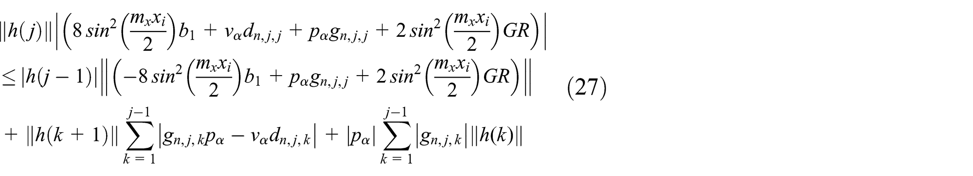
Nevertheless, using the recursive, we have

$$\begin{array}{cc}\multicolumn{1}{c}{}& \Vert h\left(j\right)\Vert \left|(8\mathrm{si}{n}^2\left(\frac{m_x{x}_i}{2}\right)b_1+v_{\alpha }{d}_{n,j,j}+p_{\alpha }{g}_{n,j,j}+2\mathrm{si}{n}^2\left(\frac{m_x{x}_i}{2}\right)\mathrm{GR})\right|\hfill \\ \multicolumn{1}{c}{}& <\left|h\left(0\right)\right|\Vert (-8\mathrm{si}{n}^2\left(\frac{m_x{x}_i}{2}\right)b_1+p_{\alpha }{g}_{n,j,j}+2\mathrm{si}{n}^2\left(\frac{m_x{x}_i}{2}\right)\mathrm{GR})\Vert \hfill \\ \multicolumn{1}{c}{}& +\Vert h\left(0\right)\Vert \sum _{k=1}^{j-1}|g_{n,j,k}{p}_{\alpha }-v_{\alpha }{d}_{n,j,k}|+\left|p_{\alpha }\right|\sum _{k=1}^{j-1}\left|g_{n,j,k}\right|\Vert h\left(0\right)\Vert \hfill \\ \multicolumn{1}{c}{}& =\Vert h\left(0\right)\Vert \{\Vert (-8\mathrm{si}{n}^2\left(\frac{m_x{x}_i}{2}\right)b_1+p_{\alpha }{g}_{n,j,j}+2\mathrm{si}{n}^2\left(\frac{m_x{x}_i}{2}\right)\mathrm{GR})\Vert \hfill \\ \multicolumn{1}{c}{}& +\sum _{k=1}^{j-1}|g_{n,j,k}{p}_{\alpha }-v_{\alpha }{d}_{n,j,k}|+\left|p_{\alpha }\right|\sum _{k=1}^{j-1}\left|g_{n,j,k}\right|\}\hfill \end{array}$$

Then

$$\begin{array}{cc}\multicolumn{1}{c}{}& \frac{\Vert h\left(j\right)\Vert }{\Vert h\left(0\right)\Vert }<\frac{\{\Vert (-8\mathrm{si}{n}^2\left(\frac{m_x{x}_i}{2}\right)b_1+p_{\alpha }{g}_{n,j,j}+2\mathrm{si}{n}^2\left(\frac{m_x{x}_i}{2}\right)\mathrm{GR})\Vert +\sum _{k=1}^{j-1}|g_{n,j,k}{p}_{\alpha }-v_{\alpha }{d}_{n,j,k}|+\left|p_{\alpha }\right|\sum _{k=1}^{j-1}\left|g_{n,j,k}\right|\}}{\left|(8\mathrm{si}{n}^2\left(\frac{m_x{x}_i}{2}\right)b_1+v_{\alpha }{d}_{n,j,j}+p_{\alpha }{g}_{n,j,j}+2\mathrm{si}{n}^2\left(\frac{m_x{x}_i}{2}\right)\mathrm{GR})\right|}\le 1\hfill \end{array}$$

Thus

$$\frac{\Vert h\left(j\right)\Vert }{\Vert h\left(0\right)\Vert }<1$$

This completes the proof.

Numerical simulations

In this section, we present some numerical simulations of the solution when N = 100 and for different values of α and β. In this simulation, the following theoretical parameters are chosen: $L=10,R=5,G=10,{\sigma }_x={\sigma }_t=0.96$ . For the initial and boundaries conditions, we have the following: $V(x,0)=\cos (x)$ , $V(0,t)=\text{sin}(t)$ , and $V(5,t)=\cos (5+t)$ . The numerical simulations are depicted in Figures 1–4 as function of time and space for different values of α and β. In these simulations, we use the software Mathematica.

Figure 1.

Numerical simulation for β = 1.96 and α = 0.95.

Figure 2.

Numerical simulation for β= 1.66 and α= 0.65.

Figure 3.

Numerical simulation for β= 1.46 and α= 0.45.

Figure 4.

Numerical simulation for β= 1.26 and α= 0.25.

From the figures, we observe a significant variation in the numerical solutions as the coupled values of α and β decrease.

Conclusion

The aim of this work is to propose the numerical version of the Caputo–Fabrizio fractional derivative with order between 1 and 2. The second-order special approximation is therefore achieved using the Crank–Nicolson approach. An error analysis of this approximation is presented in detail. In order to be consistent, we propose a transition between the ordinary derivatives to Caputo–Fabrizio fractional derivative. Making use of this transition, we modified the model underpinning the RLC circuit as function of space and time. The new model is solved numerically and numerical simulations are presented for different values of α and β.