Sage Journals: Discover world-class research

Abstract

Introduced in this article is a 1:15 brine model experiment rig with an actual large space building as the research object, which provides different concentration brine for a simulation of the stratified air conditioning in the steady-state flow field featured with columnar air supply in the bottom, heat source on the ground, the central air return, and air exhaust from roof in a large space. According to the similarity theory, it is concluded that the similarity criterion numbers applied here are Reynolds number (Re) and Archimedes number (Ar) for designation of experiment rig size, choosing device type, and confirming experiment condition. In the designation of key components of experiment rig, the application of automation control makes brine recovery and recycling in the process; designation of electrical control system makes a centralized control of experiment start–stop and the adjustment of the pipeline flow, realizing automation in the whole experiment process. Particle image velocimetry testing technology is used to get velocity vector field of air return mouth area in the model under various working conditions, and also proper orthogonal decomposition method is applied to analyze flow field structure of air return mouth area and reconstruct it. Consequently, we can get a kinetic energy ratio of return air entrainment of lower air-conditioning section and upper non-air-conditioning section in large space. Experiments show that under the conditions of same air supply, indoor environment temperature difference, and height and direction of return air inlet, fastening the speed of return air suction, the entrainment of flow field around it strengthens accordingly. The entrainment of return air inlet has more kinetic energy in the lower air-conditioning section than the upper non-air-conditioning section.

Keywords

Under-floor air supply in the large space brine model experiment return air inlet particle image velocimetry proper orthogonal decomposition

Introduction

In order to create a more comfortable and energy-saving indoor thermal environment, the stratified air-conditioning mode with downside air supply is increasingly applied to large space building. The air distribution of this kind of air-conditioning system is the lateral air supply from lower wall of the building, along with the thermal plume formed from indoor heat source, the central return air of a building, and air exhausted from the roof.

So far, analysis of indoor air distribution on the lateral air supply from lower part of large space building mostly focuses on the supply air, plume flow, and related characteristics.^1,2 However, they have less concern on return air entrainment.

Stratified air conditioning in large space is generally divided into upper un-air-conditioning area and lower air-conditioning area. Stratified air-conditioning featured with under-floor air supply and middle air return shall appear entrainment phenomenon due to the middle air return, and airflow in the un-air-conditioning space shall flow into the lower ordinary space which leads to an increase in energy consumption of air-conditioning system.

However, since the air return of air-conditioning system is set in the lower part of the building in the non-air-conditioned area and air-conditioning distinction interface, resulting in the obvious difference between the interface air movement with the traditional vents air supply system. We cannot take advantage of the current specification stratified air-conditioning load forecasting method for calculating the convective heat transfer loads in the interface. For large space with low side-wall air supply and middle side-wall air return stratified air-conditioning load, the convective heat transfer of the upper part of the non-air-conditioned area to down air-conditioned area is one of the key issues in the load study. But it is hard to have an accurate conformation of the shifted heat.

Therefore, the air return system in air conditioning with low side-wall air supply and middle side-wall air return need to analyze its air stream movement, to provide a theoretical reference for the convective heat transfer load calculation in interface. To accurately determine the convective heat transfer of the upper part of the non-air-conditioned area to down air-conditioned area caused by the building middle side-wall air return entrainment, we first need to solve return airflow and its entrainment motion flow field structure and energy distribution problem. Therefore, this article analyzes the air return flow and its entrainment motion flow field structure and energy distribution.

In this article, liquid model experiment method is used to solve this problem. In order to have a quantitative analysis of return air entrainment volume and its shifted heat, the authors put forward the concept of “return air kinetic energy proportion,” which is defined as the kinetic energy ratio between return air entrainment in the upper ordinary space and in the lower air-conditioning space.

At present, model experiment is mainly used in the research of indoor airflow. In the field of liquid experimental studies, the most notable study was the displacement natural ventilation conducted by Linden et al.³ in 1990, proposing first the natural ventilation model “emptying filling box,” expounding flow mechanism of the displacement natural ventilation indoor and verifying the theoretical expressions of flow velocity and single-point source and single-line source of thermal stratification interface location through liquid model experiment. O Auban et al.⁴ applied liquid model experiment to simulate the indoor steady-state flow field under the ground plate air supply. In 2006, NB Kaye and PF Linden⁵ used liquid model experiment to simulate motion of three fluids with different densities in the same tank at the same time, studied the motion characteristics of fluctuation corresponding to the cold and hot air jet, and analyzed the interaction of jet in opposite movement. J Oca et al.⁶ used liquid model experiment to study the greenhouse ventilation, during which they carried out related research specially for the liquid model experiment to evaluate the influence of Re on the experiment and reassessed range of Re that can ignore influence of viscosity on the experiment.

Wang Lei⁷ used the method of liquid model experiment to study the natural ventilation driven by heat pressing. Liang Yun and Wang Xin⁸ applied liquid model experiment device to conduct relevant theoretical and experimental research on nozzle jet interaction with thermal plume in large space building; Liu Chuanju and Zheng Wen⁹ used liquid model experiment to study the performance evaluation index of the terminal device of displacement ventilation.

In the large space building, because of its complex internal structure, special thermal environment, and changing indoor air movement, the direct test of the flow field of the actual building becomes very difficult.³ Liquid scale model experiments⁴ can solve this problem, which is one of the most commonly used methods to study air movement. It uses brine with a concentration moving in clean water, which can effectively simulate non-isothermal gas in the chamber flow state. By testing liquid fluid velocity distribution, the actual building can be obtained indirectly in the distribution of airflow velocity.

Based on an actual large space building as the prototype, this article sets up the liquid model experiment rig. Particle image velocimetry (PIV)¹⁰ is used to capture the instantaneous velocity vector field in the test area in time; however, what PIV captured is only the instantaneous velocity vector field, presenting the flow trend in the flow field. It cannot directly reflect the structure of flow field and be applied on energy analysis. This article introduces the method of the proper orthogonal decomposition (POD). Using the optimal orthogonal basis, POD can breakdown the structure of the flow field in different scales into complete sequence according to the size of energy and re-rank them, so as to realize the effective separation and reconstruction of flow field. POD is widely used in all kinds of flow field structure; Yang Dong et al.¹¹ used this method to predict the structure of flow field of thermal stratification under the horizontal wind in limited space. Others such as plate boundary layer flow,¹² channel flow,¹³ and so on all used the POD method to conduct analysis of flow field structure.

By introducing POD method, this article reprocesses the velocity vector field of return air inlet area captured by PIV. In the steady-state conditions of stratified air conditioning in the form of low supply and middle return in large space, this article makes a preliminary study of entrainment flow field of return air inlet of the model and calculates the kinetic energy ratio of return air inlet entrainment between upper un-air-conditioning space and lower air-conditioning space.

Designation and set up of experiment rig

The experiment theory

Regarding the gymnasium of University of Shanghai for Science and Technology as the prototype, the building is 20 m long from the east to the west, 14.8 m wide from south to north and 18 m high. The columnar air supply outlet in the lower part and air return inlet in the middle part are evenly distributed on the north and south side walls, as shown in Figure 1. The columnar air supply outlet is half cylindrical tuyere consisted of half cylinder of diameter of 600 mm nested in the 1250 × 600 × 600 mm³ sized cuboid, the tuyere surface is a square grid of about 73% void fraction, and return air inlet is circular seam-type tuyere, 400 mm diameter.

Figure 1.

(a) Gymnasium of University of Shanghai for Science and Technology and (b) columnar under-floor air supply outlet and air return inlet in the middle part.

According to the similarity theory, flow phenomenon of air in the prototype and liquid in model must be the same kind of physical phenomenon, which can be described with the same control equations. As long as the control equations are the same, two kinds of motion can achieve similarity. Air and liquid fluid motion can be described by control equations consisted of the continuity equation, mass conservation equation, and energy conservation equation. Thus, this article applies the similarity criterion Reynolds number Re and Archimedes number Ar.

Brine model experiment applied in this article has self-simulation, so a guarantee of Archimedes number Ar is all right according to the thought of approximate modeling.^14–16 The similar measuring scale of designed experiment is shown in Table 1.

Table 1.

Similar measuring scale.

Characteristic quantity	Architecture archetype	Fluid mold	Similar scale form	Ratio
Geometric dimensioning	H_s	H_m	L_H = H_s/H_m	15 (selection¹³)
Density (temperature) difference	ΔT_s/T_s₀	Δρ_m/ρ_m₀	L_T	1
Velocity	U_s	u_m	L_U = (L_H)^1/2	3.87
Time	T_s = 1/u_s	T_m = 1/u_m	L_t = L_H/L_U	3.87
Under-floor air supply flow	Q_s	Q_m	L_Q = L_U × L_H² × β_s/β_m	1788.86
Buoyancy flux	$B_{s} = (W_{s} g_{s} β) / (c_{p} ρ_{s 0})$	$B_{m} = (Q_{m} g_{m} Δ ρ_{m}) / ρ_{m 0}$	L_B	871.42

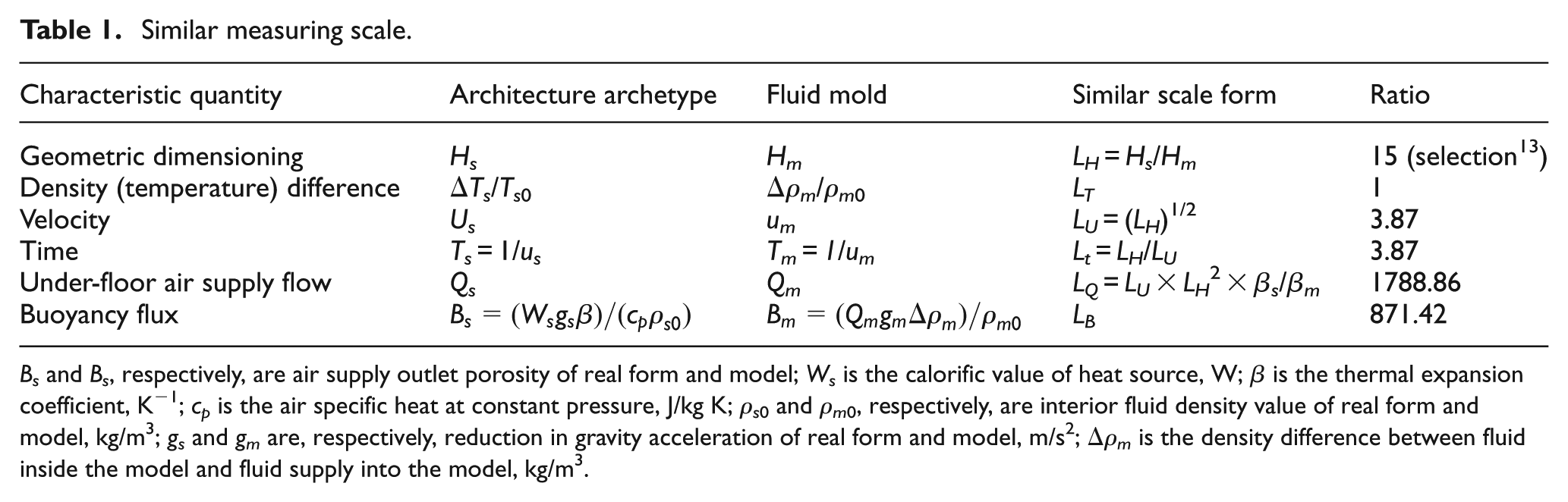
B_s and B_s, respectively, are air supply outlet porosity of real form and model; W_s is the calorific value of heat source, W; β is the thermal expansion coefficient, K⁻¹; c_p is the air specific heat at constant pressure, J/kg K; ρ_s₀ and ρ_m₀, respectively, are interior fluid density value of real form and model, kg/m³; g_s and g_m are, respectively, reduction in gravity acceleration of real form and model, m/s²; Δρ_m is the density difference between fluid inside the model and fluid supply into the model, kg/m³.

Large space model is designed in accordance with the ratio 1:15 scale; in the experiment rig, there are only simulations of one under-floor air supply outlet of columnar model, one inlet, one air outlet, and heat source plume device; system flow chart is shown in Figure 2, and Figure 3 shows the physical diagram of the experiment rig.

Figure 2.

System flow chart of brine experiment of stratified air conditioning in the form of low supply–middle return in the large space.

Figure 3.

Physical map of brine experiment of stratified air conditioning in the form of low supply–middle return in the large space: (a) one-piece tank of brine mixing, water, and water supply and (b) the main environmental water tank.

Brine of the 14th brine tank simulates blast. Brine concentration is determined by a subsequent experiment condition; the size of the concentration is determined by the size of a hand-held conductivity meter. In all, nine brine supply pumps provide power to make the brine to flow through the outlet of the seventh column directly into the 6th environment tank.

Return air is provided power by the 13th power pump to extracting aqueous from the 6th environment tank through the 11th model return air into 15th backwater tank.

The water of 1st thermal plume water tank simulates actual heat source which flows from the 4th plume inlet into the 6th environment tank.

Bench design brine recovery and recycling systems are used to ensure brine state of constant flow and constant density in the 14th salt water tank. The brine of 17th brine tank is fed continuously into the 19th high water tank which set overflow tank and the excess brine through the overflow tank back to the 17th brine tank to make a constant water level high and a constant elevation to ensure constant flow of the brine inflowing to the 16th brine deployment tank.

The dilute brine in the 15th backwater tank overflows into the 16th brine deployment tank. Smart conductivity meter (29) is used for real-time monitoring brine density of the 16th brine deployment tank. The density signal is through No. 27 proportional–integral–derivative (PID) controller feedbacks to the 28th electric actuator valve to change the valve opening to control brine flow, which flows from the 19th high water tank into the 16th brine deployment tank and to ensure the density values required by brine in the 14th brine tank. Meanwhile, conductivity meter is installed in the export of 14th water tank to monitor density real time.

Design and production of brine supply and return device

Model with the column low side air supply tuyere

By geometric scale C_H = 15 reduced scale, the size of the model with the column low side air supply tuyere: diameter of 20 mm, 83 mm high for the semi-cylindrical sleeve embedded in a size 83 × 20 × 12 mm rectangular, the low side outlet using three-dimensional printing production technology, in the form of a circular aperture, the aperture is 5 mm, as shown in Figure 4.

Model with air return

The actual air return, with a diameter of 400 mm round tuyere, locates in the low side air supply tuyere just above the 4.5 m height. Also according to the air return of model, C_H = 15 design geometric scale size, as shown in Figure 5.

Simulation heat transfer with water plume trap and injection port

In experiment, the water plume injects from the bottom of the brine model to simulate the heat transfer of prototype with the large space lower portion air-conditioned area.

Figure 4.

The column low side air supply tuyere of the (a) actual building and (b) model.

Figure 5.

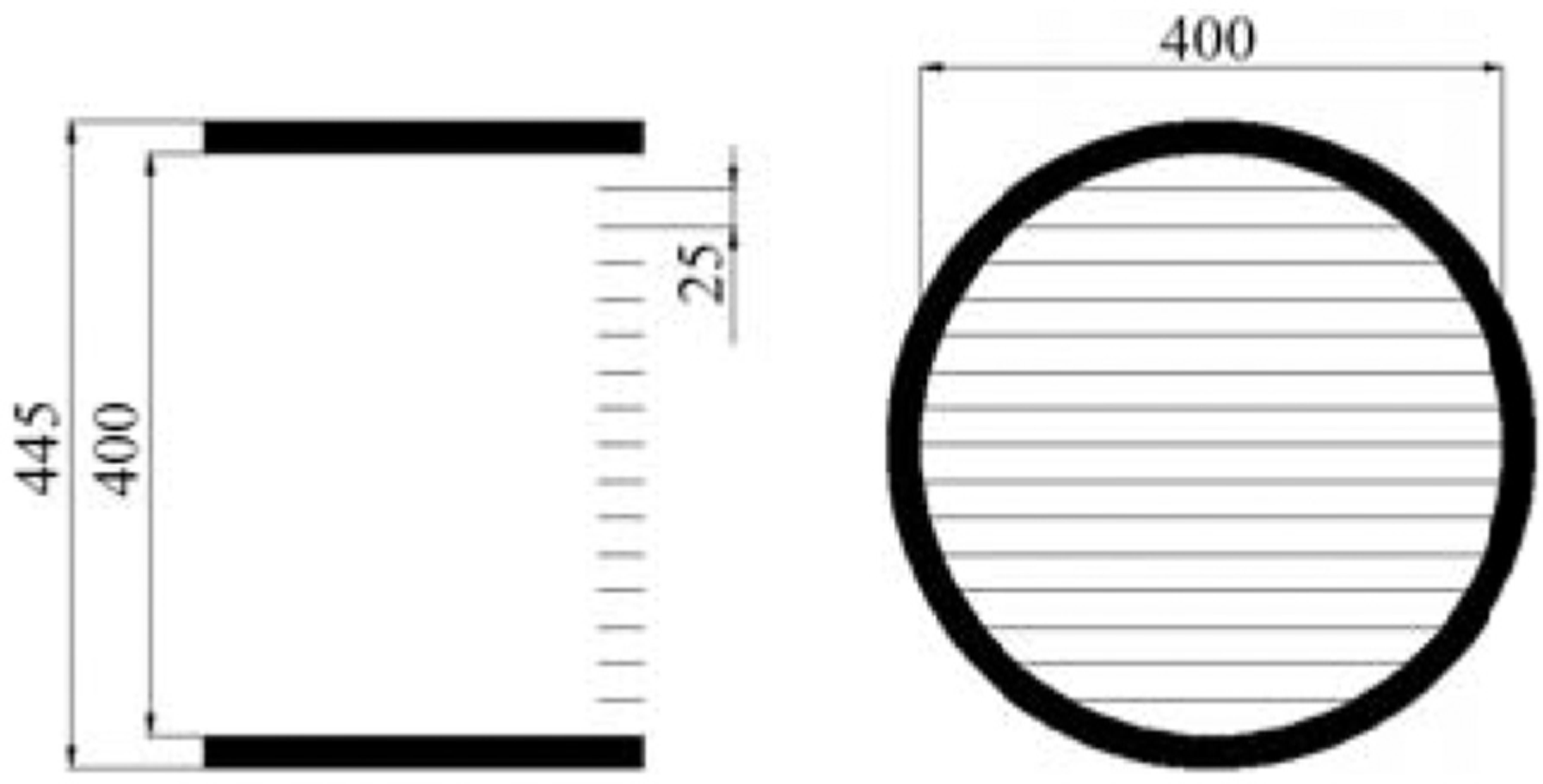
Side view (left) and front view (right) of air return.

Plume injection port role is to reduce the initial momentum generated when the water is injected into the water tank, so the water can be fed into the tank at a lower speed and more evenly spread in the tank. Design plume inlet of size 400 × 400 × 40 mm, opening a pore diameter of 10 mm, is shown in Figure 6.

Figure 6.

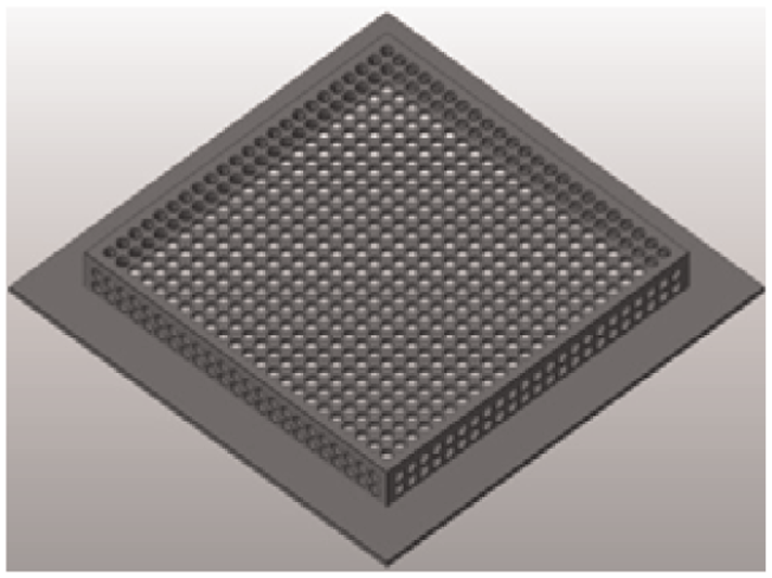
Plume filler component.

Discussion on key points of brine model experiment rig designation

Cyclic running. In order to achieve the steady state of stratified air-conditioning system in the form of low supply–middle return in large space, a certain density of brine is applied for simulating air supply to environmental water tank in the process of simulation. To simulate the fresh and return air mixing of the air-conditioning system, dilute brine (return) is used for recovery and recycling, making recycled dilute brine and prepared concentrated brine mixed and deployed to the brine density value of air supply simulation through the density meter and PID controller.

Closed-loop control designation in piping system. Testing table is set up with five pipes of simulation of under-floor air supply, middle air return, air exhaust from the top, heat source on the bottom, and the fresh and return air mixed, making electromagnetic flowmeter, inverter, and water pump as a closed-loop control system in the pipeline; before operation of experiment, the traffic percentage is set in the frequency converter, when running experiments; in the operation of experiment, electromagnetic flowmeter transmits the digital signal-measured flow rate value to the inverter and then PID algorithm of the inverter is calculated to change the pump motor speed, which adjusts pipe flow to setting percentage flow rate value. At the same time, in the process of operation, as the pipeline flow changes, frequency converter is ready to fine-tune flow through the PID algorithm to ensure each pipe always stay at the specified flow value.

Designation of electrical control system. Testing table is set up with five pipes of simulation of under-floor air supply, middle air return, air exhausted from the top, heat source on the bottom, and the fresh and return air mixed. In order to solve instability caused by separated start and adjustment of flow of the pipe, all the closed-loop control circuits are connected to the electrical control cabinet, directly controlling start–stop of control system and traffic percentage setting through start–stop button on the panel and inverter panel on it. Thus, it can realize centralized control of the whole system.

The heat of actual large space building is transferred by the ground heating, building envelope, and roof; however, the heat sources of simulated heat centralized at the bottom of the model, flowing into the water tank in the form of a plume, overflowing from overflow portion of the upper water tank, and entering into the overflow recycling bins to ensure water balance in the water tank.

In order to simulate vertical temperature distribution of the stratified air conditioning, the determination of the initial density of main water tank experiment needs to consider the average temperature of the air-conditioning section under the actual working conditions. For example, the average temperature of the actual upper un-air-conditioning section is 38°; the initial density of the main water tank is set according to 38°, which means the beginning density of the return water is set according to 38°. Backwater need to drop the density from 38° to 27° as in air-conditioning zone. Therefore, known at the beginning of the experiment conditions are water supply, water return, and water density, which are determined by supply and return air parameters of the air-conditioning system in the actual working condition, and the density of the main water tank is determined by average temperature state of ordinary section in actual working condition.

If the density of the main water tank is set according to 38° which is higher than the air-conditioning designed temperature (e.g. 27°), it equals to indoor internal heat source for the tank bottom-air-conditioning area. The sum of this internal heat source and plume heat can be considered the initial indoor cooling load, which is equal to the amount of cold air-conditioning system provided. So, the plume and water flow at the experiment beginning can be determined. As the temperature of the main tank is mixed with supply water and temperature slowly reduces to 27°, the initial indoor cooling load is carried by the cold air-conditioning system. At the moment, the need of cooling capacity of air-conditioning system equals to thermal plume heat, and then, the plume and water flow can be determined.

Other parameters of air-conditioning system in the experiment rig are carried out in accordance with the similar scale conversion.

Experimental verification of indoor vertical temperature distribution

Experiment condition

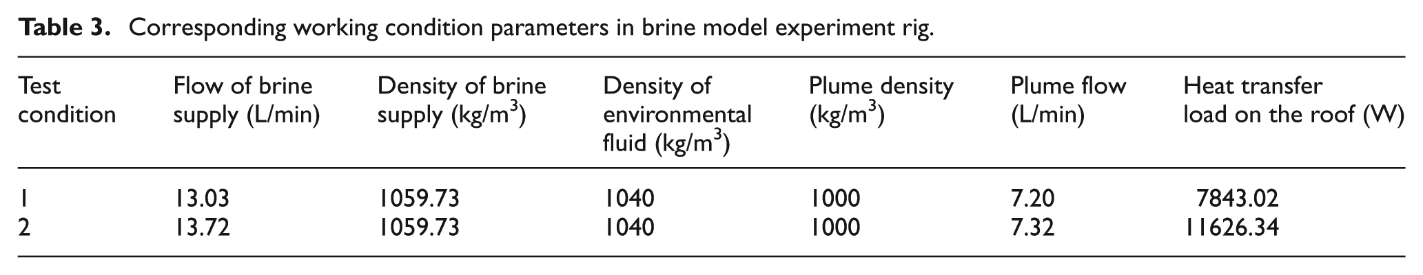
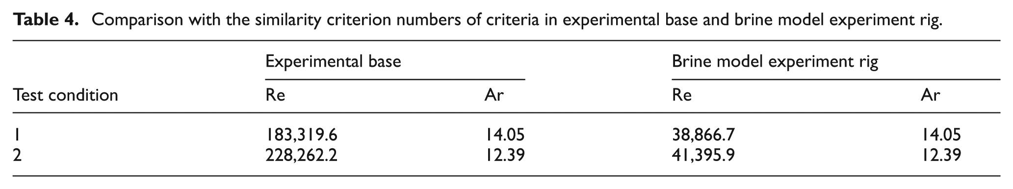
In this article, the experiment selected two field-measured data in the large space experimental base in the summer of 2010 and acquired experimental parameters in the model experiment rig after similar analysis, as is shown in Tables 2 and 3. The values of Re and Ar of experimental base and brine model experiment rig are shown in Table 4. By comparing indoor vertical temperature distribution in large space experiment base and brine model experiment rig, the model results can be used to simulate the indoor temperature distribution and the airflow movement in the form of low supply–middle return in the actual large space building.

Table 2.

Working condition parameters in experimental base.

Test condition	The actual supply air temperature (°C)	Return air temperature (°C)	Air capacity (m³/h)	Air speed on the surface of under-floor air supply (m/s)	Outdoor temperature (°C)	Integrated temperature (°C)
1	22.7	30.9	9349	0.38	35.1	41.4
2	19.5	30.7	11641	0.47	37.9	46

Table 3.

Corresponding working condition parameters in brine model experiment rig.

Test condition	Flow of brine supply (L/min)	Density of brine supply (kg/m³)	Density of environmental fluid (kg/m³)	Plume density (kg/m³)	Plume flow (L/min)	Heat transfer load on the roof (W)
1	13.03	1059.73	1040	1000	7.20	7843.02
2	13.72	1059.73	1040	1000	7.32	11626.34

Table 4.

Comparison with the similarity criterion numbers of criteria in experimental base and brine model experiment rig.

	Experimental base		Brine model experiment rig
Test condition	Re	Ar	Re	Ar
1	183,319.6	14.05	38,866.7	14.05
2	228,262.2	12.39	41,395.9	12.39

PIV testing technology takes pictures and get low side-wall air return convergence zone velocity vector information in different wind speeds of saline model experiments. One goal of this article is to calculate, the height of the air return to the interface, the indoor upper part non-air-conditioned area enter air volume to building central vertical air return, which need to get back to the air return convergence zone velocity vector information in order to gain access to the proportion of non-air-conditioned area air volume to the total air return volume of wind accounted for air return.

In the experimental base, three vertical temperature measuring lines are uniformly distributed along the center line from east to west and the one from north to south of the building. Totally, 18 testing points are arranged for measuring temperature on the vertical direction in every 0.4 m interval of the area below 2.4 m and every 0.5 m interval of area above 2.4 m. This article adopts thermocouple to obtain the data regarding monitoring and acquisition of temperature constantly; corresponding positions of internal brine tank of actual line are distributed on density measuring points; eight testing points are arranged for measuring density on the vertical direction in every 0.8 m interval of the area below 2.4 m and every 1.0 m interval of area above 2.4 m. Conductivity meter is adopted to obtain the data regarding the monitoring and acquisition of the density.

Analysis on experiment result

By comparing experimental value of vertical temperature distribution to measured values, it can be concluded that the temperature distribution inside the model is consistent with vertical temperature distribution in actual building, as is shown in Figure 4. Under the condition of the same height, maximum temperature difference appears at 0.87 m with temperature difference Δt 0.49°C. By comparing the vertical temperature distribution in the actual building to the model building, it can be concluded that the slopes of temperature trends are basically identical. Under the condition of the same height, maximum temperature difference appears at 3.465 m with temperature difference Δt 1.18°C. The average temperatures of actual building and air-conditioning area in model building are, respectively, 28.85°C and 29.09°C, whereas the average temperatures of actual building and the ordinary section are, respectively, 35.41°C and 35.09°C. The measured temperature of return air in steady state of model building is 31.18°C and in actual building 30.9°C. Figure 7 is the comparison chart of temperature distribution in vertical direction in model building and actual building under working condition 2. Horizontal temperature of the model is relatively uniform. Under the condition of the same height, maximum temperature difference appears at 1.665 m with temperature difference Δt 0.31°C. By comparing the vertical temperature distribution in the actual building to the model building, it can be concluded that the slopes of temperature trends are basically identical. Under the condition of the same height, maximum temperature difference appears at 0.87 m with temperature difference Δt 1.6°C. The measured temperature of return air in steady state of model building is 30.9°C and in actual building 30.7°C. By comparing the indoor vertical temperature distribution in experimental base of large space and brine model building, it can be concluded that model results of brine model experiment rig can be used to simulate the indoor temperature distribution and the airflow movement of the low supply–middle return in the actual large space building.

Figure 7.

Comparison chart of temperature distribution in vertical direction in model building and actual building under the test conditions 1 and 2.

Return air entrainment kinetic energy ratio analysis on the airflow organization form as low supply–middle return

POD

POD has proved to be an effective method for identifying dominant features and events in experimental and numerical data. It has the added advantage of effectively compressing or summarizing large quantities of data so that the most useful information about the physical processes occurring may be extracted. It was first introduced in the context of turbulence by Lumley,¹⁷ but was suggested independently by several researchers before this, including Kosambi (1943), Loe’ve (1945), Karhunen (1946), Pougachev (1953), and Obukhov (1954) (see J Kostas et al.¹⁸ for more details on these references). POD also goes by the names Karhunen–Loe’ve decomposition, principal component analysis (PCA), singular value decomposition (SVD), empirical eigenfunction decomposition, among others. Its uses include random variable analysis, image processing, signal analysis, data compression, process identification and control in chemical engineering, oceanography, even psychology, and economics (see J Kostas et al.¹⁸ for references on each discipline).

When performing a POD of a flow, we are looking for fluid motions that contribute most to the energy of the flow (defined as the mean square fluctuating value of the flow variable under investigation). The decomposition (akin to a Fourier series decomposition) results in a set of modes that represent an average spatial description of structures containing most of the energy and which are predominantly associated with large-scale structures. They do not necessarily have to correspond to coherent structures. The modes may also correspond to events in the flow that contribute the most, in a statistical sense, to the energy of the flow.

Flow field analysis, application, and physical significance of the method of the POD

The POD is a method used to decompose complex flow field into several mode of basic features, which is then used to analyze basic mode one by one to get the primary and secondary structures of the original complex flow field. From the perspective of energy analysis, POD contains the coherent structure and its energy of the flow field to identify the structure of the larger energy in the flow field; from the perspective of mathematical analysis, the POD is a set of optimal orthogonal coordinate system in the flow field function space that was obtained by computing; the flow field vector collection has the biggest projection on each coordinate axis of this set of coordinates.¹⁹

In this article, two-dimensional POD is used to analyze the velocity vector field of the vertical plane in return air inlet, and the kinetic energy in the flow field is associated with the velocity vector. Suppose you have X instantaneous velocity vector field, and each velocity vector field can be used as a x₁ X x₂ two-dimensional matrix V, while the element value V_mn in matrix is represented the location of the flow field parameters, indicating the correlation of X instantaneous flow field elements covariance matrix of AX X X is expressed as

A_{ij} = \frac{1}{x_{1} x_{2}} \sum_{m = 1}^{x_{1}} \sum_{n = 1}^{x_{2}} V (v_{mn}, t_{i}) V (v_{mn}, t_{j})

(1)

where V_mn is the flow field parameter of a specific position, and speed is measured in m/s; t_i and t_j are the time nodes of flow velocity vector.

Applying orthogonal decomposition on the covariance matrix, matrix eigenvalue alpha 1, alpha 2, …, alpha X and the corresponding eigenvector {aX} can be obtained, so each POD mode can be calculated as follows

φ^{i} = \sum_{j = 1}^{k} α_{j}^{i} V^{j}

(2)

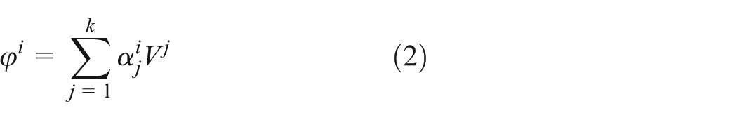
where $α_{j}^{i}$ is the jth element corresponding eigenvector {aⁱ} of aⁱ; V_j is the original flow field parameters.

Among them, the size of the eigenvalues represents the energy (kinetic energy) contained in the corresponding POD mode, and POD mode is rearranged according to the size of eigenvalues. Then, the POD mode with larger energy is low-order mode as the dominant flow field structure in the flow field.

Then, orthogonal decomposition is used to combine the whole sequence mode and finally the original flow field can be reconstructed

V_{t}^{i} = \sum_{n = 1}^{x} α_{i}^{n} φ^{n}

(3)

Through refactoring POD mode flow field, the energy and flow state contained in the main flow structure of flow field can be more intuitive observed. This article uses POD algorithm combined with the MATLAB program to calculate the eigenvalue of velocity vector field.

Test condition

Test conditions are described in Table 5.

Table 5.

Test condition.

Working condition	Flow of watersupply (L/min)	Flow of water return (L/min)	Height of return air inlet (m)	Direction of return water	Density of water supply (kg/m³)	Density of environment (kg/m³)	Plume flow (L/min) and density (kg/m³)
1	7.99	7.99	0.3	Horizontal	1013.13	1003.23	0.88, 1000
2	11.82	11.82
3	15.97	15.97
4	19.97	19.97
5	23.64	23.64

Results and discussion

The selection of shooting area of velocity vector diagram

Because this article studies proportion of kinetic energy of return air entrainment in low supply–middle return system in large space (considering the centralized line of return air inlet of the model as the boundary of upper ordinary section and lower air-conditioning section), it is important to select a representative film region. Viewing the center of return air inlet as the centralized line, 10 × 10, 13 × 13, 15 × 15, 16 × 16, 17 × 17, 18 × 18, and 20 × 20 (unit: cm), these seven areas are selected to test the inlet velocity vector field in the test condition 1, and POD method is applied to calculate kinetic energy ratio change trend of upper and lower areas. Figure 8 is the kinetic energy ratio of the upper and lower areas of 1-order mode and all 25-order modes in the above seven areas. The upper and lower of the 10 × 10 areas have a relatively maximum kinetic energy ratio (85.47%) due to the domination of velocity vector in the core region of the return air inlet which balanced the kinetic energy in the upper and lower areas. The upper and lower of the 20 × 120 areas have a relatively minimum kinetic energy ratio (66.15%), which is due to the chosen area border near the rising plume and the increase in kinetic energy because of the lower regional velocity field by plume disturbance. The kinetic energy in areas of 13 × 13, 15 × 15, 16 × 16, 17 × 17, and 18 × 18 is relatively close. The energy ratio of 1-order mode is between 71.82% and 80.01%, the energy ratio of whole sequence of 25-order mode is 87.3%–91.1%. So, the proportion of the kinetic energy calculated in the selection of PIV shooting area within this period can reflect kinetic energy of upper and lower areas of the return air entrainment stratification plane. This article selects 17 × 17 region to conduct flow structure analysis and for kinetic energy calculation.

Figure 8.

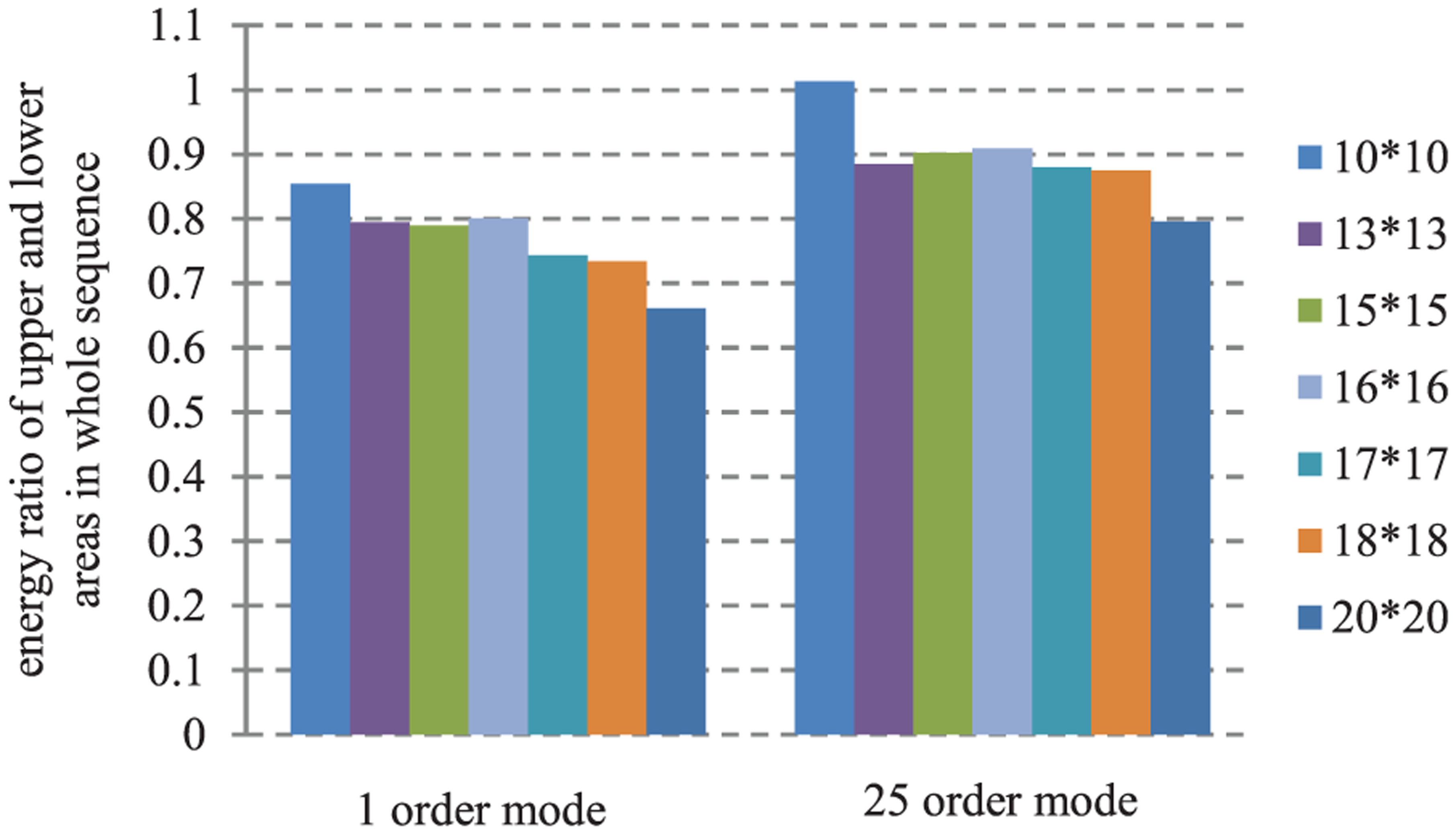
Energy ratio of upper and lower areas in whole sequence of 25-order mode and 1-order mode.

Transient vector field

Figure 9(a) and (b) shows the transient velocity vector field of 17 × 17 region in test conditions 1 and 2 in interior flow field mode at its steady state. Figure 9 shows that due to the return air suction effect, area around return air inlet form a confluence flow field with high regional speed and high attenuation of air speed. When air speed reduces to a certain area, vortices begin to produce. Return air velocity in test condition 1 is bigger than in test condition 2 and the confluence area of working condition is relatively large.

Figure 9.

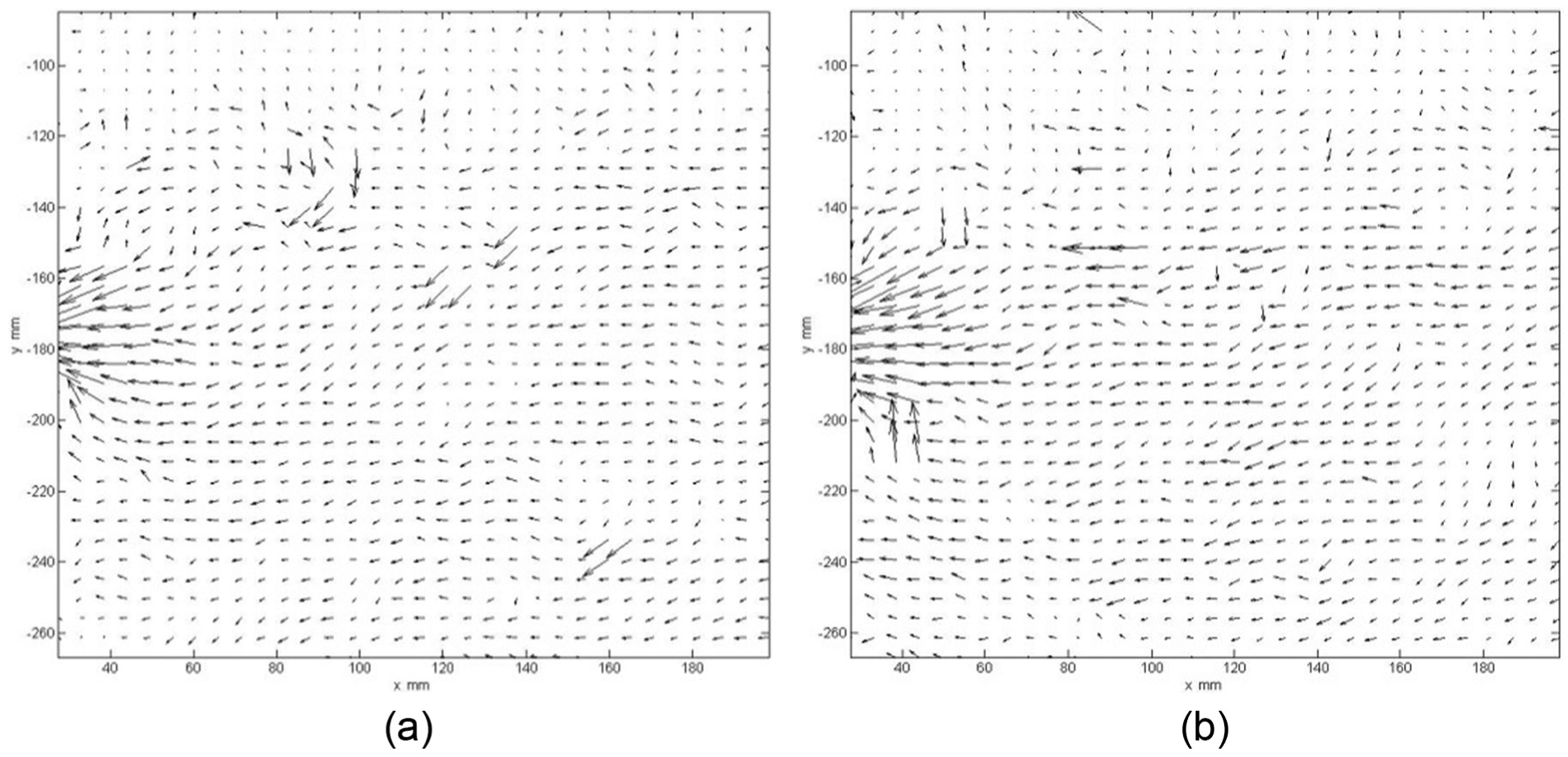
(a) Test condition 1 and (b) test condition 2.

POD modal analysis

This article selects 25 transient velocity fields with uniform time intervals after flow field reached stable as an object of POD analysis. Figure 10(a) and (b) presents the 1- and 25-order modes in the flow field of the test condition 1, it can be seen that the dominant 1-order mode mainly is the large-scale structure formed from confluence flow near return air inlet, while 25-order mode is small-scale structure in flow field. We can see the similar rule in Figure 10(c) and (d).

Figure 10.

The flow field after proper orthogonal decomposition reconstruction: (a) 1-order mode in test condition 1; (b) 25-order mode in test condition 1; (c) 1-order mode in test condition 2; and (d) 25-order mode in test condition 2.

Figure 11 shows corresponding POD spectrum in the test conditions of 1–5, conditions 1 and 2 are taken as examples for analysis. It can be seen that 1-order mode occupies most of the kinetic energy in flow field, 74.97% and 55.81%, respectively. Compared to 1-order mode, the kinetic energy proportion of 2- and 3-order mode significantly decreases, as 2- and 3-order mode in the test condition 1, respectively, account for 2.53% and 3.35% of the total kinetic energy flow field; 2- and 3-order mode in the test condition 2, respectively, account for 5.31% and 4.22% of the total kinetic energy flow field, the higher order mode reflects the smaller vortex structure, and randomness of movement direction is heavier. As mode order is high, large-scale vortex will break and separate into small-scale vortex which will finally cause kinetic energy dissipation. From the proportion of kinetic energy of 1-order mode, it can be seen that the dissipation proportion of kinetic energy in transferring to high-order mode in the test condition 1 is significantly greater than that in the test condition 2. This shows that the return air suction speed increase causes more and more small-scale eddies and strengthens the entrainment of the surrounding flow field.

Figure 11.

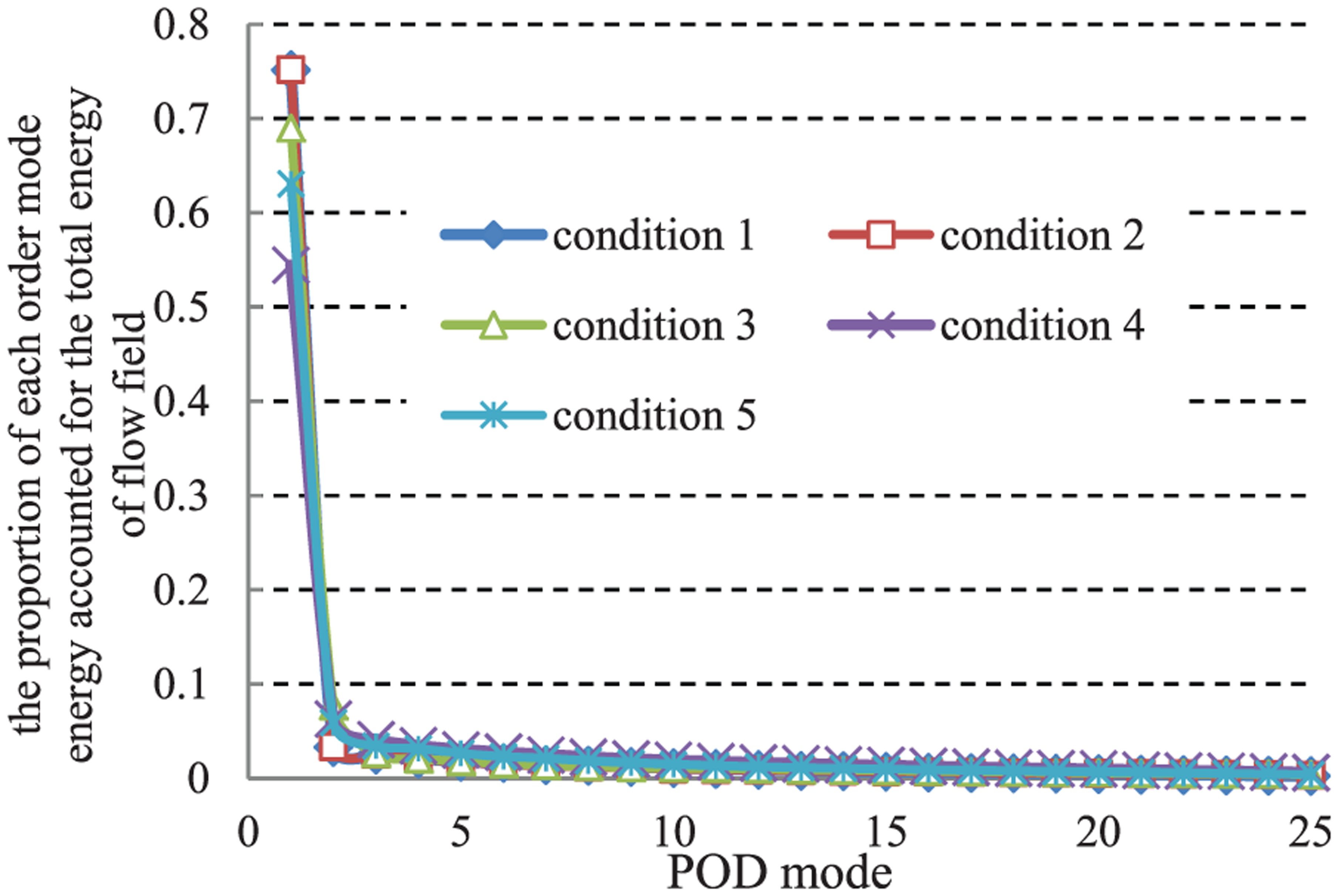
The proportion of each order mode energy accounted for the total energy of flow field.

Upper and lower regional energy ratio analysis

Figure 12 is the ratio of the kinetic energy of area above the boundary and area below it in different order modes. Analysis is still conducted in the test conditions 1 and 2. As can be seen in it, the kinetic energy ratio of the upper area and lower area of each order model in the test condition 1 is larger than that in the test condition 2. The return air inlet pumping speed of the test conditions 1 and 2 is 0.36 and 0.63 m/s, respectively; when the return air speed increases by 75%, the kinetic energy ratio of area above the boundary and area below it decreases by 22.36% for low-order mode (1-order mode), while the kinetic energy ratio of area above the boundary and area below it increases for high-order mode (14-order mode and above) such as 25-order mode, the kinetic energy ratio of area above the boundary and area below it decreases by 43.8%. It can be illustrated that in the same condition of air distribution, indoor environment temperature, and height and direction of return air inlet, the increase in return air suction speed strengthens the horizontal flow force and increases the generation of layered interface vortex, which increases the kinetic energy and also explains the return air suction speed increase. Compared with the area above the boundary, return air inlet entrainment in the area below the boundary has larger kinetic energy. When suction speed of the return air inlet is 0.36 m/s, the upper area accounts for 42.65% of the total kinetic energy in 1-order mode; when suction speed of the return air is 0.63 m/s, the upper area accounts for 36.73% of the total kinetic energy in 1-order mode.

Figure 12.

The ratio of the kinetic energy of area above the boundary and area below it.

Conclusion

In this article, a 1:15 brine model experiment rig is set up with an actual large space building as the research object, which conducts a simulation of the stratified air conditioning in the steady-state flow field featured with columnar air supply in the bottom, heat source on the ground, the central air return, and air exhaust from roof in a large space. PIV testing technology is used to get velocity vector field of air return inlet, and POD method is applied to the analysis of flow field structure of return air inlet entrainment and its proportion of the kinetic energy of area above the boundary and area below it. The results show the following:

By calculating the energy ratio of the upper and lower areas of return air inlet, it is concluded that area of 13 × 13–18 × 18 cm is the mostly reflecting PIV shooting areas for the kinetic energy of return air entrainment on areas both above and below the boundary.

Because of return air entrainment effect, area surrounding return air inlet forms a confluence flow field with larger regional speed and higher speed of attenuation. As attenuation of air speed reaches a certain area, vortices begin to produce. As return air entrainment speed increases, confluence area expands with high speed.

In the confluence flow field of return air inlet, 1-order mode is mainly the large-scale structure formed from confluence flow near return air inlet, 2-order mode has few large-scale structures transferring into a small-scale structure, while 25-order mode is small-scale structure in flow field. Of the total energy in the flow field, 1-order mode energy is dominated, and energy attenuation is rapid from 2-order mode.

As entrainment speed of return air increases, more and more small-scale eddies generate and entrainment of the surrounding flow field strengthens.

In the same condition of air distribution, indoor environment temperature, and height and direction of return air inlet, the increase in return air suction speed strengthens the horizontal flow force and increases the generation of layered interface vortex, which increases the kinetic energy and also explains the return air suction speed increase. Compared with the area above the boundary, return air inlet entrainment in the area below the boundary has larger kinetic energy.

Footnotes

Academic Editor: Hyung Hee Cho

Declaration of conflicting interests

The author(s) declared no potential conflicts of interest with respect to the research, authorship, and/or publication of this article.

Funding

The authors would like to thank the National Natural Science Foundation of China (Grant Nos. 51108263, 51278302) and Hujiang Foundation of China (D14003) for financial support for this research.

References

Huang

Liu

Zou

. Experimental study on thermal environment in large-space building with low sidewall air supply. J Southeast Univ 2010; 26: 270–273.

Wang

Huang

. The fluid mechanics of ventilation system generated by buoyancy and momentum sources in a single room. J Harbin Instit Technol 2010; 14: 531–535.

Linden

Lane-Serff

Smeed

. Emptying filling boxes: the fluid mechanics of natural ventilation. J Fluid Mech 1990; 212: 309–335.

Auban

Lemoine

Vallette

. Simulation by solutal convection of a thermal plume in a confined stratified environment: application to displacement ventilation. Int J Heat Mass Tran 2001; 44: 4679–4691.

Kaye

Linden

. Colliding turbulent plumes. J Fluid Mech 2006; 550: 85–109.

Oca

Montero

Antón

. A method for studying natural ventilation by thermal effects in a tunnel greenhouse using laboratory-scale models. J Agr Eng Res 1999; 72: 93–104.

Wang

. Experimental study of displacement-style natural-ventilation driven by hot-pressing. Harbin, China: Harbin Institute of Technology, 2006.

Liang

Wang

. Large space horizontal and vertical flow cold model experimental study on the mutual motion of liquid jet. Shanghai, China: University of Shanghai for Science and Technology, 2012.

Zheng

Liu

. Experimental study of displacement ventilation device at the end of the performance evaluation indexes. Master’s thesis, Tongji University, Shanghai, China, 2008.

10.

Adrian

. Particle-imaging techniques for experimental fluid-mechanics. Annu Rev Fluid Mech 1991; 23: 261–304.

11.

Yang

Zhu

Huo

. Horizontal wind effect of thermal stratification in a confined space POD analysis of flow field structure. J Chongqing Univers 2013; 36: 121–126.

12.

Aubry

Holmes

Lumley

. The dynamics of coherent structures in the wall region of a turbulent boundary layer. J Fluid Mech 1988; 192: 115–173.

13.

Liberzon

Gurka

Tiselj

. Spatial characterization of the numerically simulated vorticity fields of a flow in a flume. Theor Comput Fluid Dynam 2005; 19: 115–125.

14.

Cai

Long

. Fluid pump and fan. 5th ed. Beijing, China: China Architecture and Building Press, 2009, pp.270–284.

15.

. Basic theory and method of model test. Xi’an, China: Northwestern Polytechnical University Press, 1989, pp.51–63.

16.

. Similarity method and its application. Beijing, China: China Machine Press, 1995.

17.

Lumley

. The structure of inhomogeneous turbulent flows. In: Yaglam

Tatarsky

(eds) Proceedings of the international colloquium on the fine scale structure of the atmosphere and its influence on radio wave propagation. Moscow: Nauka Publishers, 1967, pp.166–178.

18.

Kostas

Soria

Chong

. The proper orthogonal decomposition in the analysis of turbulent flows. Annu Rev Fluid Mech 2005; 25: 539–575.

19.

Qiu

Bai

Hua

. The proper orthogonal decomposition, and agent-based modeling method for prediction of flow field. Acta Aeronaut Astronaut Sin 2013; 33: 1249–1260.

Research on the kinetic energy ratio of return air entrainment in the form of low supply–middle return in the large space of brine experiments

Abstract

Keywords

Introduction

Designation and set up of experiment rig

The experiment theory

Design and production of brine supply and return device

Discussion on key points of brine model experiment rig designation

Experimental verification of indoor vertical temperature distribution

Experiment condition

Analysis on experiment result

Return air entrainment kinetic energy ratio analysis on the airflow organization form as low supply–middle return

POD

Flow field analysis, application, and physical significance of the method of the POD

Test condition

Results and discussion

The selection of shooting area of velocity vector diagram

Transient vector field

POD modal analysis

Upper and lower regional energy ratio analysis

Conclusion

Footnotes

Declaration of conflicting interests

Funding

References