Computational fluid dynamics simulation and geometric design of hydraulic turbine draft tube

Abstract

Any hydraulic reaction turbine is installed with a draft tube that impacts widely the entire turbine performance, on which its functions are as follows: drive the flux in appropriate manner after it releases its energy to the runner; recover the suction head by a suction effect; and improve the dynamic energy in the runner outlet. All these functions are strongly linked to the geometric definition of the draft tube. This article proposes a geometric parametrization and analysis of a Francis turbine draft tube. Based on the parametric definition, geometric changes in the draft tube are proposed and the turbine performance is modeled by computational fluid dynamics; the boundary conditions are set by measurements performed in a hydroelectric power plant. This modeling allows us to see the influence of the draft tube shape on the entire turbine performance. The numerical analysis is based on the steady-state solution of the turbine component flows for different guide vanes opening and multiple modified draft tubes. The computational fluid dynamics predictions are validated using hydroelectric plant measurements. The prediction of the turbine performance is successful and it is linked to the draft tube geometric features; therefore, it is possible to obtain a draft tube parameter value that results in a desired turbine performance.

Introduction

The draft tube is a necessary component installed in a reaction turbine, and it is the last component in the flux stream over the hydraulic turbine. Its main function is to convert the remaining kinetic energy into static pressure allowing an orderly flux, and this causes an increasing effective head for the runner component and therefore better turbine efficiency. The draft tube has an irregular geometry; thus, the geometric definition is dictated by a large number of parameters that must be selected carefully according to their influence on the draft tube hydraulic behavior. The draft tube construction is another feature to consider, which requires a large amount of excavation, and then an improved compactness design will result in a reduction of costs. Traditionally, the draft tube design is based on simplified analytic methods, experimental prototypes, and recently due to the increase in computer parallel computing, by numerical methods such as computational fluid dynamics (CFD). ¹ Due to their relevance on the turbine performance, there is a great interest in developing new methodologies to design and analyze the draft tube.^2,3 Similar studies were performed using geometric parameterization^1,4,5 based on one or more parameters that defined a single draft tube geometric feature (i.e. the cone angle or elbow radius). Hellström JGI et al. ¹ carry out CFD computations to evaluate an original and redesigned draft tube. With their CFD computations, they did not find any improvements in the pressure recovery of the two draft tube geometries. But their predictions did not agree with the experimental results, so they recommended to include the runner in CFD computations and to use adequate boundary conditions. In their computations, they evaluated just two draft tube geometries, solving three-dimensional Reynolds Averaged Navier Stokes (RANS) equations and $k-\epsilon$ turbulence model. In this work, a draft tube design–analysis methodology based on a CFD is proposed. The implemented CFD modeling solves the flow in the turbine guide vanes, runner, and draft tube. First, the CFD computations were validated using power and efficiency measurement from the hydraulic site. Also the boundary conditions were applied according with pressure measurement at the hydraulic power plant. In order to analyze the effect of the draft tube geometry, 256 draft tubes were constructed and meshed using a homemade algorithm that is based on a mathematical expression whose coefficient defines most of the draft tube geometric features. The effect of different flow conditions also was taken into account through 10 different opening positions of guide vanes. The post-process analysis of the CFD results presented are focused on behavior patterns of the key hydraulic variables (pressure, velocities, P, U, V) through the draft tube which are important to design and for performance evaluation. All methodology presented in this article describes a way to tackle both draft tube issues: design and analysis.

Geometric parametrization

The draft tube under study belongs to a Francis turbine with specific speed n_s  = 265.8 and power capacity of W = 38.5 MW. The Francis turbine is located in San Miguel Soyantepec, Oaxaca, México. The turbine base line parameters are listed in Table 1. The guide vane is composed by 24 blades, while the runner has 13 blades. Figure 1 shows the turbine components considered in the simulation. In order to minimize the computational cost, the spiral case domain is not included in the CFD computations. This decision may not take into account some flow effects; however, main losses occur at runner exit and draft tube, so the selection of the components was decided by the balance between the impact on turbine efficiency (hydraulic losses) and the computational cost. The spiral case is the component that has less hydraulic losses in the turbine assembly ⁶ and has a considerably volume that is proportional to computational cost.

Table 1.

Turbine prototype baseline parameters.

	Feature		Feature
Axe	Vertical	No. guide vanes	24
Type	Francis	No. runner blades	13
Water head	50 m
Flow	90 m3/s
Power	4.59 × 107 W
Speed	180 rpm

Figure 1.

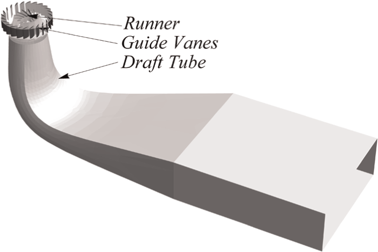
Modeled turbine components.

Due to the static diffusion task and the suction performed in the turbine by the draft tube, its shape is given by a crescent cross-sectional area, typically from a circle, defined by the runner outlet diameter, which is transformed to a rectangle. The typical shape of the draft tube can be decomposed into three zones: cone, elbow, and diffuser (Figure 2(b)). The cone zone handles the swirling flow delivered by the runner and starts the diffusion task. The elbow transforms the vertical flux direction to a horizontal direction. This zone is responsible for the complexity of the flow phenomena ⁷ being that the elbow receives a swirling flow in the cone and then drastically modifies the flow’s direction which causes flow detachment. Finally, the diffuser zone ends the diffusion task providing an organized flux to the outlet. Due to the flux phenomena induced by the draft tube (principally by the elbow zone), the draft tube losses impact downstream to the runner which makes the runner and the draft tube responsible for most of the hydraulic losses.

Figure 2.

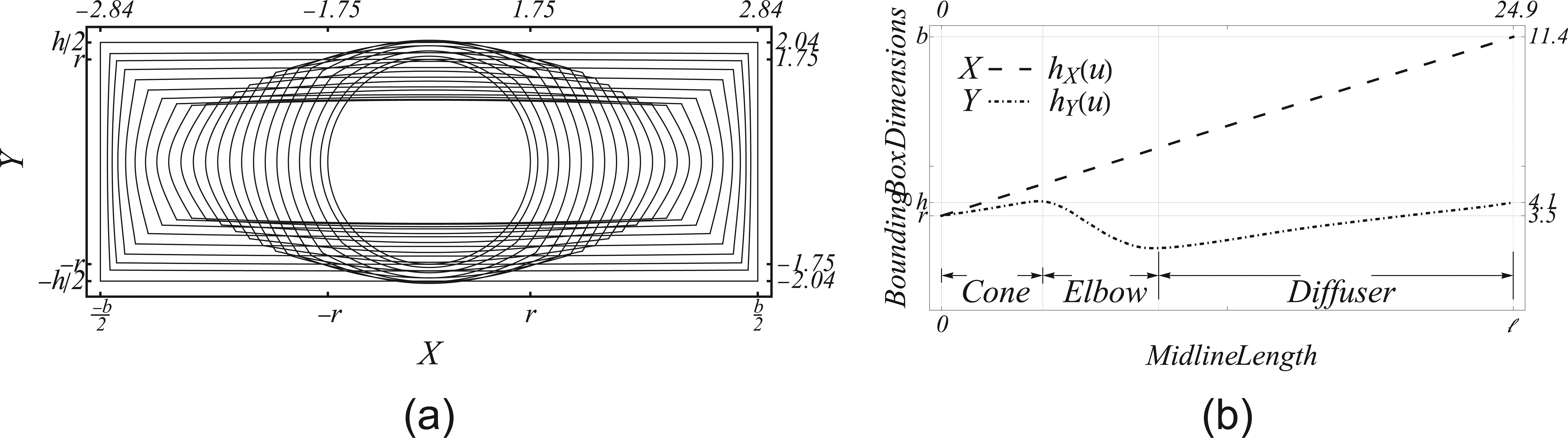
Draft tube main dimensions: (a) typical cross-section area transition, plane XY and (b) cross-section variation.

The draft tube usually splits in the diffuser zone using one or more piers that have primarily structural purposes, ² due to this reason and to simplify and reduce the geometric modeling, the draft tube without piers is considered in this study. Therefore, the main dimensions are the inlet and outlet sizes and the transversal cross-sectional areas that are transitions between inlet and outlet. The dimensions of the cross-sectional area are presented by the bounding box dimensions of each cross-section and are shown in Figure 2(b). Observe that the bounding box dimensions at the inlet are r × r and b × h at the outlet. Figure 2(a) displays the circle–rectangle transition contained in the XY plane that is orthogonal to the draft tube midline. The total midline length is l = 24.9 m and is used as third curvilinear dimension that describes the draft tube.

The initial shape and dimensions of the draft tube displayed in Figure 2 show that in the Y-direction, the cross-sectional area is considerably reduced (due to the transition between the cone zone to the elbow zone) in a nonlinear way, and, given its properties, it can be adjusted by a function h_Y (u) that is a BSpline. ⁸ In the X-direction, the cross-sectional area is linearly increased along the draft tube length. This transition is adjusted by a linear function h_X (u). Both functions h_Y (u) and h_X (u) morphed the circular cross-section area (generally with the parametric form: cs(t) = {cos(t), sin(t)}) to rectangular cross-sectional area (defined by a piecewise parametric function rs(t)) through the length of the draft tube midline ml(u) which normally is also a BSpline that contains the rest of the draft tube dimensions. The above analytic implementations facilitate working with the geometric features of the draft tube. An inherent advantage attached to the analytic description is the resultant flexibility on the discretization process. The meshing or discretization can be performed by algebraic methods and the resultant mesh has equivalent properties for any draft tube.

The proposed modifications are focused on the cross-sectional area contained in the XY plane. The variation applied on the cross-sectional area does not imply a large increment on the draft tube total dimension, unlike a manipulation applied to the midline length or to the total cone height. Such modifications are suitable in cases that a refurbishment is required or the design is restricted by excavation volume issues. Equation (1) produces a modified draft tube set (m, n) which varies in X- and Y-directions, respectively. The (m, n) modifications are applied gradually to the draft tube, similar to that of a stone sculpt process

$$\begin{array}{c}\multicolumn{1}{c}{{\mathrm{Tube}}_{m,n}=\{h_X(u),h_Y(u)\}}\\ \multicolumn{1}{c}{+\{(\frac{m-1}{15}.\frac{3}{2}-\frac{1}{2})j(u),(\frac{n-1}{15}.\frac{3}{2}-1)j(u)\}}\\ \multicolumn{1}{c}{m=1,2,3,...,16,n=1,2,3,...,16}\end{array}$$

(1)

In the above equation, a modification is performed by the addition of the term $((m-1/15)·(3/2)-(1/2))j(u)$ or $((n-1/15)·(3/2)-1)j(u)$ to the original cross-sectional area $\{h_X(u),h_Y(u)\}$ , the $j(u)$ function is expressed in millimeter and is given in equation (2)

$$\begin{array}{c}\multicolumn{1}{c}{j(u)=-14532.1u^7+28625.2u^6-37848.4u^5}\\ \multicolumn{1}{c}{+60586.1u^4-44204.5u^3+5986.15u^2}\\ \multicolumn{1}{c}{+1387.62u}\end{array}$$

(2)

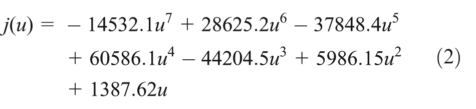
From equation (1), it is deduced that the original draft tube has the values m = 6, n = 11, and the amount of total draft tubes is 256. The draft tube set produced by equation (1) and their cross-sectional area is shown in Figures 3 and 4, and the initial draft tube is rendered in red color.

Figure 3.

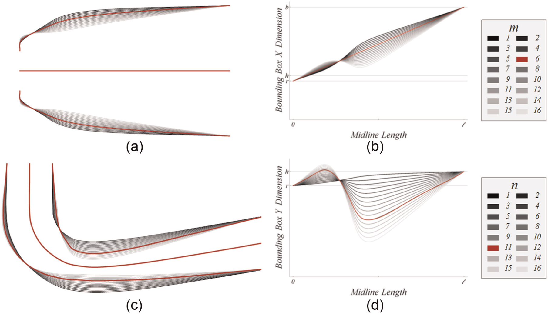
Draft tube geometric modifications: (a) equation (1) m modification, (b) X bounding box m modification, (c) equation (1) n modification, and (d) Y bounding box n modification.

Figure 4.

Modified draft tubes cross-sectional area: (a) midline length versus cross-sectional area and (b) draft tube colors.

As mentioned earlier, the component zones of the draft tube are the cone, the elbow, and the diffuser. The cone zone must be a crescent cross-sectional area, or in other words A ₁ < A ₂. The elbow cross area is the transition zone between the cone and diffuser and dependent upon the assigned elbow radius and the dimensions in the X- and Y-directions. Finally, the diffuser has a linear growing cross-sectional area. As shown in Figure 4, all characteristics are preserved in the general modifications, being that the elbow zone was most drastically modified because of its impact on the complex behavior of the flux.

CFD simulation

Given quantity of turbine operation points (10), the number of draft tubes (256), and the modeled turbine components, the computer simulation setting is extensive and the computational cost is high. An automatic scripting tool was used to establish the coupling of the Fluent^® CFD solver with the homemade mesher and the geometry generator. A brief description of the numerical modeling steps is provided below.

Discretization process

The draft tube geometry was created based on the analytical description, mentioned previously, in an own geometry design application. A structured mesh for the draft tube domain is generated by a developed software draft tube mesher. The structured mesh can provide higher accuracy in cases where the grid is aligned with the flow direction. ⁹ For the guide vane and runner computational domains, unstructured tetrahedral meshing generated by the Delaunay algorithm has been employed due to its flexibility to discretize complex geometries. The whole computational mesh consists of 637,810 elements. In all CFD simulations, the mesh dependence is important in order to check the solution convergence with respect to spatial resolution. The mesh dependence test was performed in the original draft tube case with the runner torque as the target. A coarse draft tube mesh with half number of elements of the mesh with test mesh dependence is used due to the amount of simulations (2560); however, the precision evaluated varies 5%−7% with respect to the optimum size mesh.

Solver

The entire flow field was resolved using the RANS turbulence model. The RANS models have proven to be a good approach in the draft tube flux modeling. ⁵ A standard k − ω turbulence model is employed in the simulation, the k − ω models are typically better in predicting flow separation^10,11 and offers a reasonable balance between accuracy and computational cost. In this study, the convergence criteria are set on 10⁻⁵ for all variables. Relaxation factors of 0.15–0.3 for pressure and momentum and 0.35–0.45 for other variables are applied to improve stability. A maximum of 1000 iterations is performed in each case. The script algorithmic programming include a logic sentence that exclude the results of the turbine cases which not reach the convergence criteria, some cases are the minimum or maximum simulated operation point (that corresponds to minimum or maximum guide vanes opening).

Boundary conditions

The simulations assume steady state and incompressible flow in all modeled components. The flow in the runner is established in the rotating frame of reference with an angular velocity of 180 rpm. For reducing computational cost, the guide vane and the runner were modeled only a single channel 1/24 and 1/13, respectively. Figure 5 shows the boundary zones in the turbine computational domain.

Figure 5.

Turbine boundary zones.

The inlet boundary conditions applied were the inlet pressure of 522,030 Pa at the guide vanes inlet and the flow direction. The pressure used corresponds to the turbine operation load, and the flow direction is provided by the casing outlet (−1, 0.942, 0) in cylindrical coordinates (r, θ, z). The turbine flux regulation is dictated by the opening of the guide vanes. A set of 10 guide vane domains with different degrees of opening or gap is used to model the turbine operation points. Figure 6 shows the diagram of the guide vanes opening.

Figure 6.

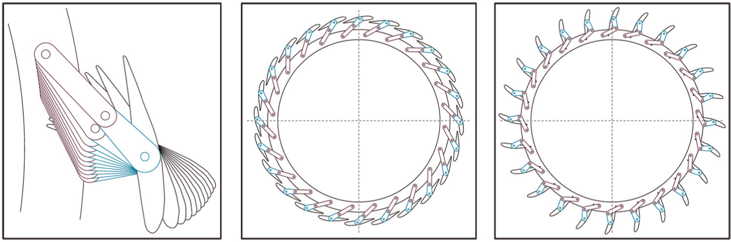
Guide vanes mechanism diagram.

With previous CFD simulations, ¹² the guide vanes opening range was approximated. Figure 7(a) shows the gap γ between the guide vanes as function of the opening angle $\iota$ , the turbine opening range is delimited by the green box. The gap is calculated by the minimum Euclidean distance between the surfaces of adjacent guide vanes. Figure 7(b) shows the location of the minimum Euclidean distance rendered by circles.

Figure 7.

Guide vanes gap: (a) opening angle $\iota$ versus gap γ and (b) gap between adjacent blades.

Multiple regions with relative motion are contained in the simulation, the mixing plane model with the mass average method ¹³ provided by Fluent^® is used for simulating flow between adjacent moving-stationary zones. Outlet boundary condition is defined by an opening at the draft tube outlet with an average relative pressure to atmospheric pressure.

Results

The maximum efficiency is the main target when a turbine is designed, and the efficiency is calculated by the energy extracted by the turbine and the available energy ratio. Equation (3) gives the turbine efficiency in terms of hydraulic variables. Another quantity of interest is the runner torque, due to the fact that this quantity indicates the energy taken by the turbine. The presented results are focused on the turbine efficiency, the runner torque and the key hydraulic variables (P, U, V) on the draft tube

$$\eta =\frac{T\omega }{\rho \mathrm{gHQ}}$$

(3)

where T is the torque, ω is the angular velocity, ρ is the density, g is the gravitational acceleration, H is the turbine head, and Q is the volumetric flow rate.

Validation with the original draft tube

The comparison between the CFD predicted efficiency and the measured efficiency serves as a validation for the CFD predictions. Moreover, the efficiency and torque are points of comparison to evaluate the improvements made by the draft tube modifications in the whole turbine performance. Figure 8 shows the performance curves for the real turbine measures and the predicted CFD quantities; x-axis shows the volumetric flow rate Q and the guide vanes gap γ given in percentage, aided with Figure 7 the guide vane opening can be estimated. In the y-axis, the runner torque T and the efficiency η are shown.

Figure 8.

CFD predictions versus plant measurements: (a) T versus Q and (b) η versus Q.

The torque and efficiency predicted by CFD show a good overall agreement with the measurement made in the hydroelectric plant (6.5% for efficiency and 4.1% for torque); the maximum efficiency peak appears nearly 74 m³/s that corresponds to γ = 51%, 228 mm, and $\iota =-1.08\mathrm{rad}$ . However, the predicted curves are offset from the real measurements, and some ways to reduce this difference are to include the spiral case in the model, to use another turbulence model or to incorporate boundary layer in the flow domain.

The (P, U, V) quantities are important to evaluate the tube performance relative to the geometric modifications; these quantities are taken for the simulation results in the draft tube cross-sections (Figure 9) that are orthogonal to the draft tube midline. The (P, U, V) CFD results in the cross-sections are presented as weighted average quantities.

Figure 9.

Draft tube cross-sections.

The (P, U, V) weighted average values in the draft tube cross-sections are shown in Figure 10 and are intended to appreciate the evolution of variables throughout the entire draft tube in all simulated operation points.

Figure 10.

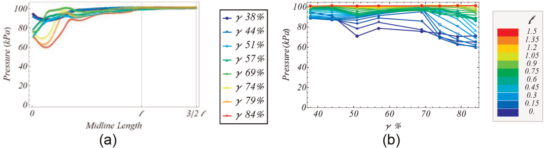
Original draft tube pressure distribution: (a) P versus l, Tube _6,11 and (b) P versus γ%, Tube _6,11.

Figure 10 shows that the maximum pressure difference is located in the inlet-cone zone, and its maximum value is reached in lower γ values. Thus, it can be seen that in the inlet-cone zone, the pressure has an inverse relationship with the opening γ; hence, the draft tube work is evidenced in this results.

Figures 11 and 12 show the tangential U and normal velocities V relative to the draft tube midline; therefore, for a correct draft tube behavior, big values of U are expected and lower V values are desirable; in addition the velocity V is linked to recirculation and energy losses. Figure 11 shows that the maximum inlet and outlet draft tube velocity U values are present in higher γ values and exhibit an approximately linear behavior (relative to γ value). Figure 12 shows that apparently the velocity V in the inlet and outlet draft tube does not have a relationship with the guide vanes opening γ, however probably does between the amplitude and frequency of the velocity V distribution waves along the draft tube.

Figure 11.

Original draft tube U-velocity distribution: (a) U versus l, Tube _6,11 and (b) U versus γ%, Tube _6,11.

Figure 12.

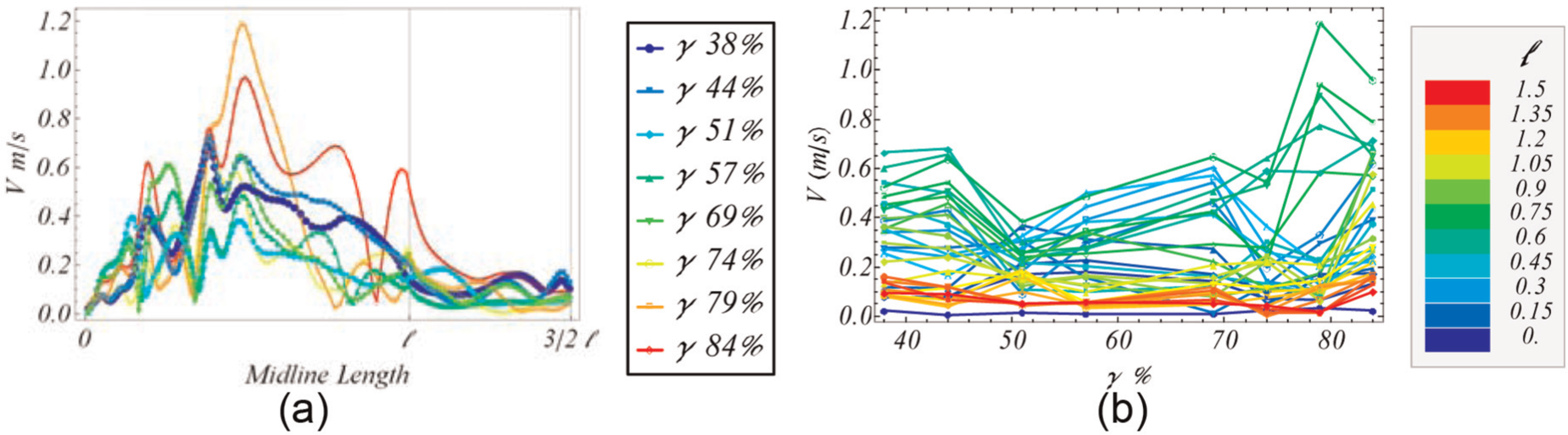
Original draft tube V-velocity distribution: (a) V versus l, Tube _6,11 and (b) V versus γ%, Tube _6,11.

Draft tube modifications

As seen in the original draft tube results, the best efficiency point (BEP) occurs approximately at 51% γ value, then the results of the draft tubes set $m=6\vee n=11$ that share m or n values with the original draft tube are presented for the same γ value. Thus, each $\mathrm{Tub}{e}_{6,n}$ and $\mathrm{Tub}{e}_{m,11}$ behavior is compared with the original draft tube behavior and can be evaluated for the geometric improvement.

In Figure 13, it can be seen that the increment of the m, n values generates higher pressure modification in the draft tube inlet and elbow zone, being more noticeable the pressure modification given by the n value. The magnitude of this pressure in the zone inlet is useful to optimize the draft tube design to prevent cavitation on the runner or select some pressure required by the runner design.

Figure 13.

Modified draft tubes pressure distribution: (a) P versus l, γ = 51%, Tube _6,n and (b) P versus l, γ = 51%, Tube_{m ,11}.

For the velocity U distributions shown in Figure 14, as the pressure distributions, the biggest changes are given by the n values; this is logical due to that the modification of sectional area is higher, but the local maximum value located in the elbow zone is more flattened in the n values than the m values. The maximum velocity U for the n values at the draft tube inlet is 7 m/s and the maximum is 7.9 m/s, and for the m values are 7.0 m/s minimum and 7.2 m/s maximum. The draft tube outlet velocities U for the n values are 1.4 m/s minimum and 1.6 m/s maximum, for the m values are 1.39 m/s minimum and 1.44 m/s maximum, both maximum and minimum inlet and outlet velocities U occur in the maximum and minimum m and n values. From Figure 14, we can see that the draft tubes with n modified values give a better flux deceleration which is a desirable characteristic in the draft tube behavior.

Figure 14.

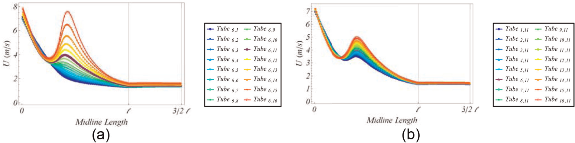
Modified draft tubes U-velocity distribution: (a) U versus l, γ = 51%, Tube _6,n and (b) U versus l, γ = 51%, Tube_{m ,11}.

The average weighted velocity V for a symmetrical swirling flow in a tube of circular or symmetrical transversal section is 0; this value is also applied when there is no swirling flow. Figure 15 shows velocity V values closest to 0 m/s in the draft tube inlet for both m and n values, implying a symmetrical swirling flow given by the impeller, this characteristic can be interpreted as a symmetrical load in the runner blades. If V values are not 0 at the draft tube inlet, the load in the blades is asymmetrical and it can produce vibrations. The velocity V distributions along the tube for m and n values have a same wave pattern, the wave amplitude varies in proportionally with the m, n values; as mentioned previously, this quantity is linked to energy losses; therefore, under this assumption, the better draft tubes are those whose m, n values result in lower V values.

Figure 15.

Modified draft tubes V-velocity distribution: (a) V versus l, γ = 51%, Tube _6,n and (b) V versus l, γ = 51%, Tube_{m ,11}.

Figure 16 shows a negligible turbine efficiency change; however, the flux in the turbine varies considerably from a m, n value to another. Therefore, the main parameter to take a design decision is the runner torque; this feature is directly linked to the power desirable in the hydroelectric plant. In Figures 17 and 18 can be seen that the m, n values slide the maximum torque peak to the left (toward lower flux values), this convert the draft tube m, n values in a flexible tool to modify the turbine point operation.

Figure 16.

Modified draft tubes efficiency: (a) η versus Q Tube _6,n and (b) η versus Q Tube_{m ,11}.

Figure 17.

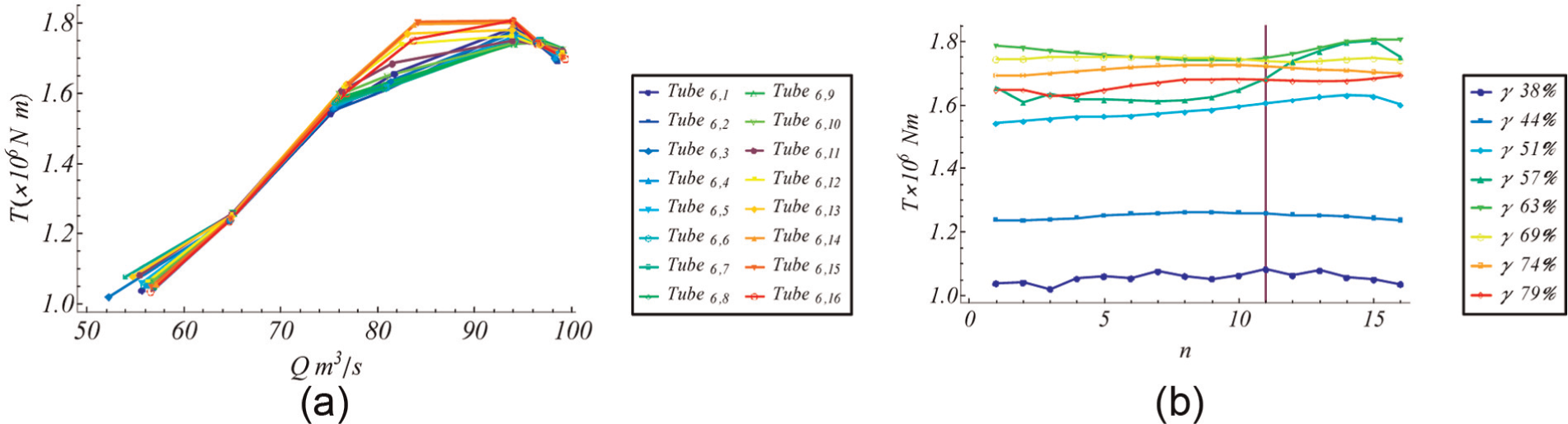
Modified draft tubes torque, Tube _6,n : (a) T versus Q and (b) T versus n.

Figure 18.

Modified draft tubes torque, Tube_{m ,11}: (a) T versus Q and (b) T versus n.

The results (P, U, V, T, η, etc.) obtained from CFD simulations corresponding to 256 turbines each with 10 operation points. The above presented results correspond to the set $m=6\vee n=11$ . The results that correspond to the set $m\ne 6\wedge n\ne 11$ are very extensive deal with numeric and graphical standard methods, given the parameters number (geometric and boundary parameters), the post-process is susceptible to deal (for analysis and optimization) with artificial intelligence systems ¹⁴ as neural networks and/or genetic algorithms, this treatment will be presented in future papers.

Conclusion

This study purposes a methodology for analysis and design of the draft tube. The analysis is based on a CFD modeling that includes the Francis turbine components: guide vane, runner, and draft tube. The draft tube analysis–design is based on a geometrical definition given by a simple mathematical expression which describes all draft tube zones (cone, elbow, and diffuser) and makes faster the parametric design without the possibility to create unrealistic draft tube geometry. The CFD predictions are consistent with the hydroelectric plant measurements (6.5% for efficiency and 4.1% for torque), and then it can be concluded that the CFD model is a good approach to analyze the turbine performance. The CFD predictions of the draft tube modifications are useful to complement the design decision focused on the hydraulic variable of interest. The draft tube used parameters, m and n, modify the performance charts providing the more suitable parameters for refurbishment issues. The draft tube geometric modifications allow to represent the draft tube wall changes associated with erosion or addition of material. The precision of the CFD model can be improved; to achieve this, it is required that the spiral case must be included, and use of more sophisticated computational algorithms to post-process the data. These features will be presented in future works.