
Abstract
The solution of the energy equation of thermo-elasto-hydrodynamic analysis for bearings by the finite element method usually leads to convergence difficulties due to the presence of convection terms inherited from the Navier–Stokes equations. In this work, the numerical analysis is performed with finite element method universally by adopting the characteristic-based split method to solve the energy equation. Five case studies of fixed pad thrust bearings have been set up with different geometries, loads, and lubricants. The two-dimensional film pressure is obtained by solving the Reynolds equation with pre-defined axial load on the pad. The energy equation of the lubricant film and the heat transfer equation of the bearing pad are handled by characteristic-based split method and conventional finite element method in three-dimensional space, respectively. Hot oil carry-over effect and variable lubricant viscosity are considered in the simulations. The results of the temperature distributions in the lubricant film and the bearing pad are presented. The possible usability of characteristic-based split method for future thermo-elasto-hydrodynamic analysis is discussed.
Keywords
Introduction
Thrust bearings are the key factor for the pumps to achieve stable performance and long-term service. Unlike journal bearings, they often operate under conditions with relatively high surface velocity (larger working radius) and substantial axial load. As a consequence, thrust bearings usually operate in the conditions where lubricant temperature rise and thermal-elastic deformation of pad surface is non-ignorable. It is important to get these lubrication properties in the designing stage. This is usually done by the thermo-elasto-hydrodynamic (TEHD) analysis.
TEHD analysis is performed by researchers on thrust bearings with different structures and operating conditions. To the knowledge of the authors, Castelli et al. 1 did the first TEHD analysis in late 1960s. They took pad deflection, temperature, and pressure into consideration. Fillon and colleagues2,3 made enormous contribution to the research of the thermal effects of bearings in the last three decades. Monmousseau et al. 4 focused on the transient simulation of a tilting-pad journal bearing back to the 1990s. Fillon and colleagues5,6 continuously made progress in the related fields. The fundamental theories of the TEHD analysis were thoroughly discussed in these works forming the base of this work.
Conventionally, in thrust and journal bearings, the lubricant film between the bearing pad and the rotating runner is modeled by (1) the Reynolds equation, which describes the pressure distribution of the two-dimensional film, and (2) the energy equation, which governs the temperature of the lubricant. The Reynolds equation can be easily discretized and solved by certain numerical methods, such as the finite element method (FEM) 7 and the finite difference method (FDM). 8 FEM is also used to calculate the deformation of the bearing pad due to both thermal stress and pressure on the pad surface. However, FEM can be applied when the governing equations of the physical system are self-adjoint. 9 Unfortunately, it is not the case when dealing with general energy equations either in the analysis of hydrodynamic lubrication or in other fluid dynamics problems. Therefore, when solving energy equations, FDM or similar methods are dominant in the numerical study of lubrication.10–12 A novel method with the name of characteristic-based split (CBS) method has been developed in the past decades. This makes it possible to use FEM to solve fluid dynamics equations, including the energy equation.
Zienkiewicz and colleagues13–15 introduced the CBS method in the 1990s. Zienkiewicz et al. 9 continued to explore the CBS method in order to solve fluid dynamics problems in different flow regimes including incompressible and compressible flow, turbulent flow, flow through porous media, and so on. According to their theory, if the computational mesh updates its position in an incremental Lagrangian manner along the dominant velocity or “characteristic,” the first-order convective terms in the Navier–Stokes (N-S) equations would disappear. Then, the remaining fluid dynamics problem can be solved by standard Galerkin spatial approximation, which is widely used in FEM approaches. CBS method allows the computational fluid dynamics (CFD) analysis to take advantages of various types of finite elements.
It is notable that some researchers also made efforts to use FEM universally in TEHD analysis. Kim et al. 7 utilized FEM techniques to analyze heat transfer effects in the fluid film of a journal bearing. However, the structure of their energy transport equation was not the same with the general energy equation inherited from the N-S equations. Brunetière and Tournerie 16 performed FEM with upwind schemes on the two-dimensional steady-state energy equation, which was an equation with convective terms as the same as the N-S equations. With the encouragement of the capability of FEM on handling complex geometry, Pahud 17 did TEHD analysis using streamline-upwind/Petrov–Galerkin (SU/PG) method developed by Brooks and Hughes. 18 Kucinschi et al. 19 employed FEM with upwind techniques in a transient TEHD analysis. Recently, Varela and Santos 20 also solved the energy equation by SU/PG formulations. It is reported that the SU/PG method achieved better stabilizing ability than the standard Galerkin procedure in steady-state FEM analysis. This SU/PG method is stemmed from the PG weighting method. So, the SU/PG method achieves the stabilizing effect by modifying the standard weighting/shape functions. Only the steady-state solution can be obtained from SU/PG method.
In this work, the CBS method is applied to solve the energy equation in hydrodynamic lubricated thrust bearing. For calculation of the heat transfer in the bearing pad, the conventional FEM is adopted. The pressure field is given by solving the two-dimensional Reynolds equation, also with FEM. Thus, only FEM, instead of the combination with other methods, is implemented.
Energy equation and CBS method
Energy equation
Assume a coordinate system, in Figure 1, with its origin on the surface of the runner and its z-axis pointing to the bearing pad.
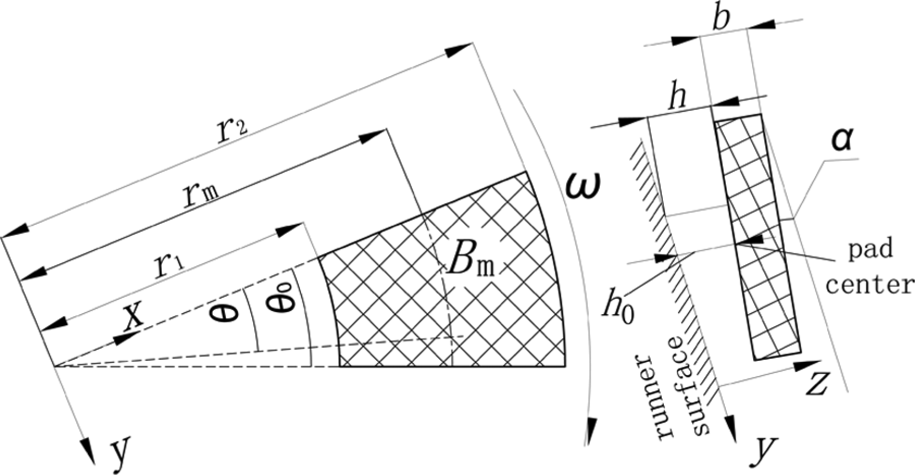
Sketch of the bearing pad and the coordinate system.
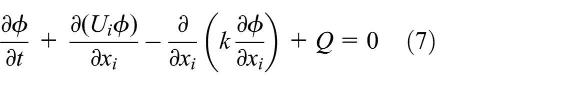
The energy equation in hydrodynamic lubrication theory is in the form of equation (1) in Cartesian coordinates
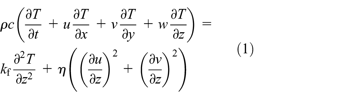
where c, k f, and η are the specific heat, the thermal conductivity, and dynamic viscosity of the lubricant, respectively. Equation (1) describes the temperature distribution of the lubricant film between the runner and bearing pad in three-dimensional space. However, it is common practice to model the pressure as two-dimensional lubricant film, which is governed by the well-known Reynolds equation. There should be some kind of transformation between the two physical fields with different dimensions of numerical treatment. This is done by modeling the velocity field. Equations (2) and (3) show the two velocity components in three-dimensional Cartesian coordinates
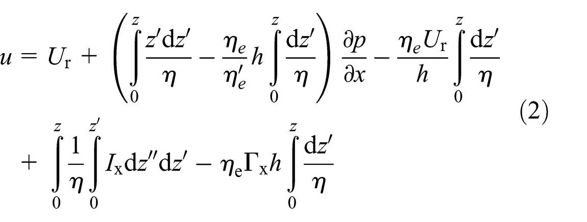

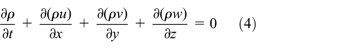
where U r(x,y,t) and V r(x,y,t) are the surface velocities of the rotating runner at specified location, p is the film pressure and h(x,y,t) is the film thickness. These formulae are based on those originally proposed by Dowson and Higginson. 21 The explanation of other symbols can be found in Appendix 2. With the help of continuity equation, equation (4), the velocity component w along z-direction can be derived
Substitute equations (2) and (3) and the derived w velocity into equation (1) and follow the procedures developed by Yang and Rodkiewicz, 22 the energy equation can be transformed into the dimensionless form, equation (5). A bar over the symbol indicates a non-dimensional quantity. The relationships between every variable and the reference quantities are listed in Appendix 3. The brief instruction on the derivation of the non-dimensional form of the energy equation is also listed in Appendix 3

where

In equation (5), Pr, Re*, and Ec are the Prandtl number, the modified Reynolds number, and the Eckert number, respectively.
The CBS method
To illustrate the implementation of CBS method, let us first consider a generalized scalar variable ϕ({
where xi
is the component of position tensor {

The time-varying unsteady solution of scalar ϕ can be found if the initial condition and the step length between the two time steps are well defined. A fundamental objective of CBS method is to derive the expression of Δϕ in terms that can, exclusively, be found at the current time step n. Zienkiewicz and colleagues9,23 explained this method in detail in their works. This is achieved by CBS method in three major procedures. Let x′i
(t) be the coordinate component along the characteristic (velocity) component U
a,i
, then ϕ = ϕ({

During the two successive time steps, the moving coordinate {


Time variance of ϕ. 9
where γ is a constant. The value ϕn
|({

And if we assume γ = 0.5, we have


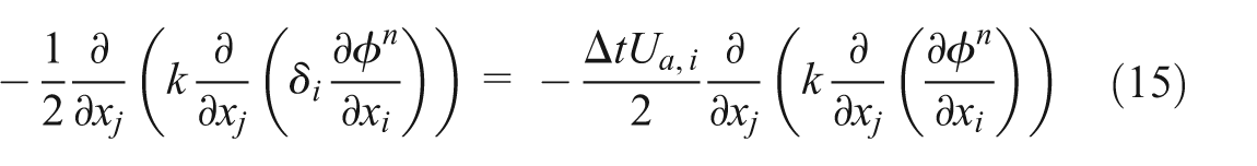
Note that distance component δi can be considered to be independent on coordinate, and then use equation (14), to approximate this distance. Then, the second term on the right-hand side of equation (12) could be written as equation (15)

In the same sense, the third term on the right-hand side of equation (11) will be

If the general diffusion coefficient, k, could be assumed to be constant, equation (15) could be transformed into equation (17)

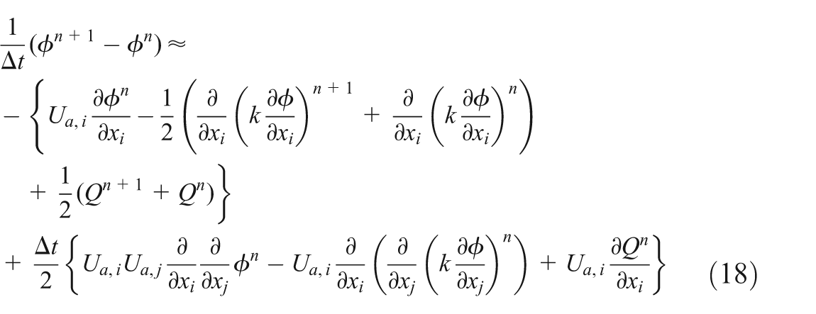
Insert equations (11)–(13) into equation (10) and considering equations (14), (16), (17), and γ = 0.5, we would have
Let us focus on the following term

The averaged characteristic component U a,i could be written as

Again, employ the Taylor expansion 9
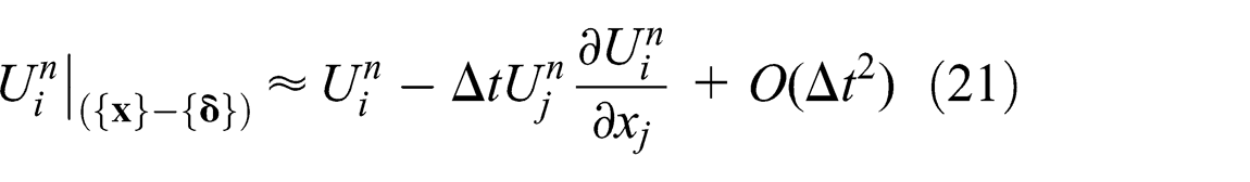
Insert equations (20) and (21) into equation (19) and neglecting the higher order terms with respect to Δt, we can write

Furthermore, the following relationship can be assumed


From equations (20) to (25), and refer equation (14), the formulation for Δϕ is expressed based on equation (18) as

In fact, because the above equation is expressed in tensor notation, the following simple relationship holds

Then, we can combine the following two terms
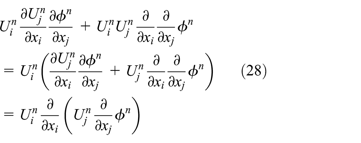
Finally, considering equation (28), equation (26) becomes

Generally, equation (29) is the same with that proposed by Zienkiewicz et al. 9 At this point, ϕn +1 can be approximated by solution at time step n. As in any other FEM implementations, the standard Galerkin spatial approximation, equation (30), can now be used to substitute the scalar unknown in equation (29)

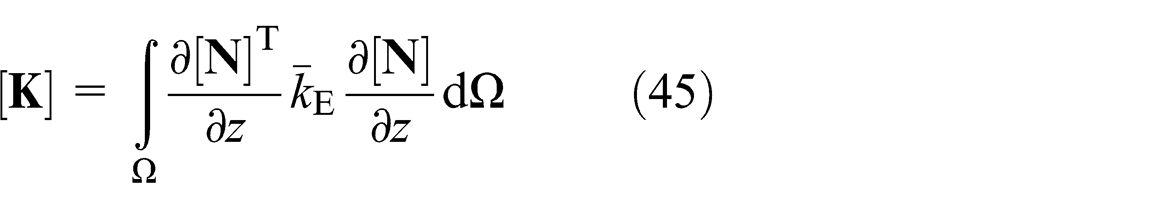
where [

where [


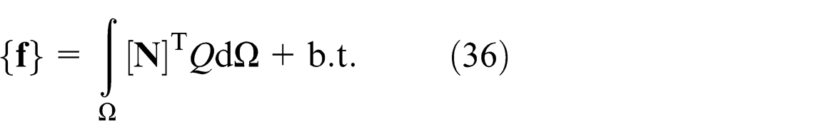

The term “b.t.” in equations (36) and (37) are the results of integration by parts and they stand for boundary conditions (Neumann boundaries). After choosing the time step length, Δt, and the initial value of
The time step length Δt has strong influence on the stability of CBS method. The largest Δt for each element is evaluated with respect to the local fluid velocity, the thermal conductivity, and the average element length (h avg), along the element’s characteristic. Zienkiewicz et al. 9 discussed several methods to determine Δt. For this work, Δt is obtained by the following procedures based on the method proposed by Zienkiewicz et al. 9 Let Pe be the Peclet number, and C c be the critical Courant number of an element


The Δt of the element is chosen to satisfy
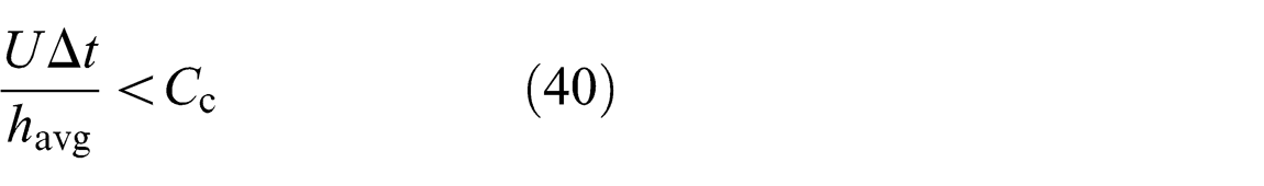
The global Δt is the smallest one among all the elements.
Remark on the energy equation
Let us rearrange the terms in equation (5) to transform it into the similar structure of equation (7). Then, we get equation (41)

where


Compared to equation (7), only the z-direction diffusion term remains. Thus, equation (34) can be written as
The temperature field now can be solved by a time-stepping manner after the selection of initial value and boundary conditions. The actual selected type of finite element and the technique of obtaining the explicit form of equation (31) by mass-lumping will be discussed in later section.
Reynolds equation and heat transfer equation
Reynolds equations
To illustrate the usability of CBS method in TEHD analysis of thrust bearing, we select the Reynolds equation utilized by Yang and Rodkiewicz. 22 Equations (46) and (47) are the Reynolds equation and its non-dimensional equivalent, respectively. The non-dimensional terms in these equations are listed in Appendices 2 and 3
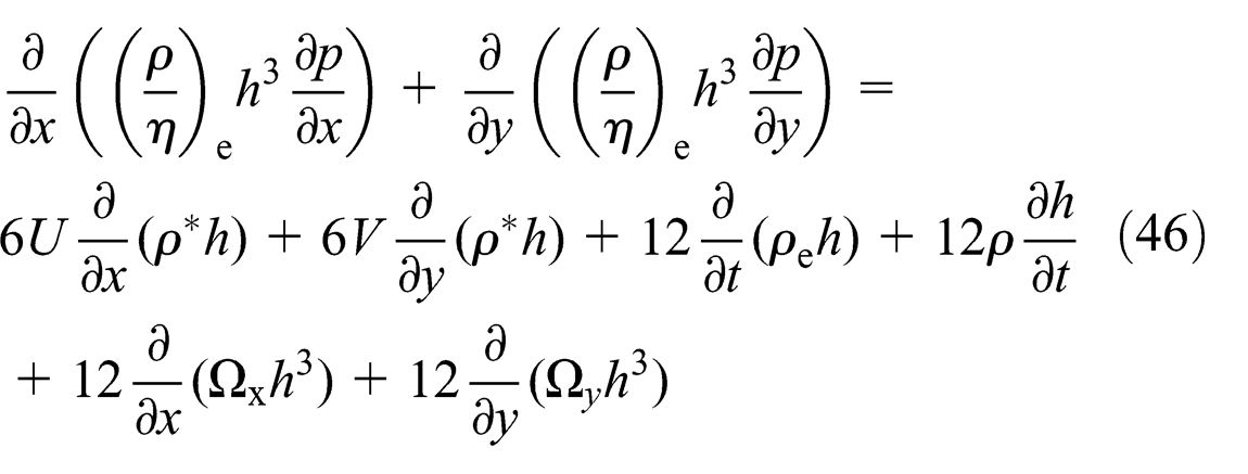

where h(x,y,t) is the film thickness, which could be expressed as equation (48) when taking the thermal-elastic deformation W into consideration

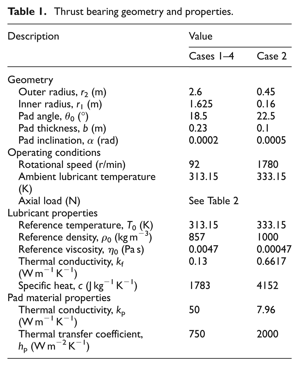
In the above expression, r(x,y) is the radius at specific location and h 0 is the film thickness at the pad center. α is one of the geometric parameters in Table 1 and Figure 1. The term W in equation (48) contains both the elastic deformation under the pressure of the lubricant film and the thermal deformation due to temperature rise in the bearing pad. It is noted here that the term W will not be considered in the demonstration computation performed later in this work.
Thrust bearing geometry and properties.
Heat transfer equation
The temperature distribution inside the bearing pad is governed by the heat transfer equation. If we assume no source term is in this equation, it reduces into the Poisson’s equation in three-dimensional Cartesian coordinates

where k p, ρ p, and c p are the thermal conductivity, density, and specific heat of the bearing pad, respectively. z p is the z-coordinate of the bearing pad with the origin on the film–pad surface. The non-dimensional form of equation (49) is equation (50). The non-dimensional reference values and procedures are listed in Appendix 3

where

where B m is the reference length and U m is the nominal average velocity (Appendix 3).
Boundary conditions
Classical Reynolds boundary conditions are used when solving the Reynolds equation. It is assumed that the bearing is fully flooded and the pressure is equal to 0 at the boundaries.
As illustrated in Figure 3, the heat flux continuity is applied at the film–pad interface. On the other surfaces of the pad, except the leading edge, a universal heat transfer coefficient h p is used. The heat exchange at the film/runner interface is set to be 0. This boundary condition will result in overestimation of the lubricant temperature. These boundary conditions could be expressed as


Surfaces and edges of the computational domain.
where T
0 is the ambient lubricant temperature. T
s is the surface temperature at faces of the bearing pad other than the film–pad interface.


where Nu is the Nusselt number defined as

The mixing effect between the hot lubricant from the exit of the preceding bearing pad and the relatively cold lubricant supply will rise the actual temperature at the leading edge of the film. This mixing effect is considered by introducing equation (56) 24 in the single-pad simulation
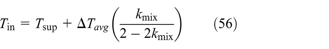
where k mix is the hot oil carry-over coefficient. In equation (56), T in, T sup, and ΔT avg are the temperature at the leading edge, the temperature of the supplied lubricant, and the circumferential temperature rise across the bearing pad, respectively. The values of T in and ΔT avg are evaluated by averaging the temperature solutions on the leading edge and tailing edge of the lubricant film. The mixing effect takes place at very film–pad temperature iteration process illustrated in Figure 4 (next section).

Solution flow chart. n 1, n 2, n 3, and n 4 are the indicators of the iteration step for different physical fields.
Some considerations should be taken before proceeding to the simulation stage. When dealing with thrust bearing with sector-shaped pads, Reynolds equation (46) is used to be defined in polar coordinates to grasp the geometry more accurately. However, in this work, we chose the equations in Cartesian coordinates to get a set of universally applicable formulations for finite element analysis. The isoparametric finite elements 25 are applied to deal with the curvature of the geometry of the bearing pad.
Although the Reynolds equation is two-dimensional, the energy equation and the temperature distribution in the bearing pad are solved in three-dimensional space. The pressure field could be considered as the so-called middle-layer 22 of the lubricant film while the temperature distribution is across the apace between the bearing pad and the rotating runner.
Single-pad simulation
Two types of finite elements are utilized for different governing equations. The eight-node tri-linear isoparametric cubic element 26 is used for discretization of the film temperature and the temperature in the bearing pad. For Reynolds equation, the four-node bi-linear isoparametric rectangular element is adopted. The shape function matrices, which are associated with those two finite element types, can be found in the work of Zienkiewicz et al. 26 The integration listed from equations (32) to (37) are calculated by Gaussian integration. 25
Five test cases are set up to evaluate the ability of the CBS method to solve the energy equation. As listed in Table 1, the bearing geometries (except the pad inclination) and properties of Cases 1–4 are the same with the large Itaipu thrust bearing studied by Wodtke et al. 27 The lubricant is oil with its dynamic viscosity at T 0 = 313.15 K (it is also the reference and oil supply temperature in the simulation) equals 0.047 Pa s. The dynamic viscosity of the oil at higher temperature is expressed by equation (57) 28,29 with β = −0.03297. Case 5 takes the geometry from the water-lubricated thrust bearing in a pump. The viscosity versus temperature property of water is described by the expression of equation (58). 30 In equation (58), η 293.15 is the dynamic viscosity of water at 293.15 K and the exponent A(T) is expressed by equation (59). The heat transfer coefficient, h p, for Case 5 is assumed to be 2000 W m−2 K−1. Case 5 is set up to test the capability of the CBS method in simulating lubrication condition with relatively lower viscosity and thinner lubricant film. The potential effects of turbulence due to the low viscosity of water and the large radius of pad geometry are simply ignored. It is emphasized that this work is made to demonstrate the usability of CBS method in solving the energy equation in thrust bearings


Two kinds of meshes are generated for the analysis. One is two-dimensional mesh for the Reynolds equation. The second is three-dimensional mesh for the energy equation. Therefore, the lubricant film in the analysis of temperature is modeled as layered structure, with several nodes and elements in the z-direction. Three-dimensional mesh is also used for the heat transfer computation. For Cases 1–4, the node number along every coordinate axis is set according to the referenced work. 27 An additional finer mesh is deployed to test the dependence of the simulation on the mesh. For Case 5, the similar mesh structure is adapted. The mesh information and the axial load settings could be found in Table 2. The axial loads of Cases 1 and 2 have the same value described in the work of Wodtke et al. 27 The hot oil carry-over coefficients, k mix, for oil-lubricated thrust bearings (Cases 1–4) are assumed to be 0.589 based on the work done by Ettles. 24 For Case 5, k mix is assumed to be 0.6.
Test case settings.

The general form of CBS method, equation (31), does not exhibit good efficiency since the solution of the full-scale linear equations should be found at every time step. And the numerical simulation maybe unstable due to some improper initial values. It is suggested that we can transform equation (31) into its explicit form, equation (60), by the mass-lumping method. Then, no actual decomposition of matrix is needed in the later iteration process

where [

in which M
l,ab is the element at Row a and Column b in matrix [
The Reynolds equation and the heat transfer equation are solved for their steady-state solutions by conventional FEM.
Several procedures are performed to solve the equations, as illustrated in Figure 4. There are two sub-iterations in the numerical solution procedures. One is the pressure–load iteration, and the other is the film–pad temperature iteration. The pressure distribution is first obtained by the initial guess of film thickness (h
0 = h
00 equals 1 × 10⁻⁴ m for Cases 1–4 and equals 6 × 10⁻⁵ for Case 5). Then, the integral of pressure over the area of the pad surface is compared with the axial load to get a correction of film thickness. An iterative process with film thickness correction continues until the axial load is balanced by the pressure integration over the pad surface. The above pressure–load iteration continues until the norm of the pressure difference of two successive iterations is smaller than the limit, e
p. Then, the velocity field is calculated by equations (2) and (3), in their dimensionless forms. In the film–pad temperature iteration, the temperature distribution is obtained through solving equation (41) by the CBS method with mass-lumping, equation (60). Then, the heat transfer equation of the pad is solved with the heat flux on the film–pad interface as the boundary condition. After the heat transfer solution, the temperature of the film–pad interface will be updated and the hot oil carry-over effect will take place. Then, the CBS method will be launched again to get the film temperature and the heat flux on the film–pad interface. The convergence of film–pad temperature iteration is achieved when the normalized difference of the successive temperature on the film–pad interface,

where {
where


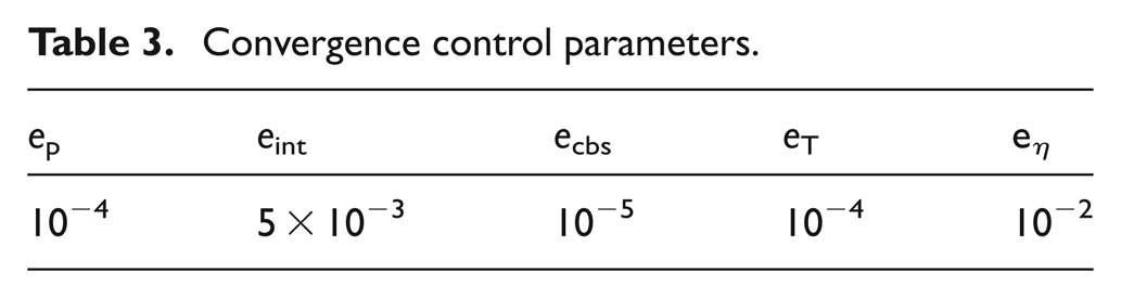
If the convergence limitations are not met, the viscosity of the lubricant will be modified by equation (57) (equation (58)) according to the local film temperature of the current solution and the whole solution procedures will be performed all over again from solving the Reynolds equation. All the convergence control parameters are listed in Table 3.
Convergence control parameters.
Results and discussion
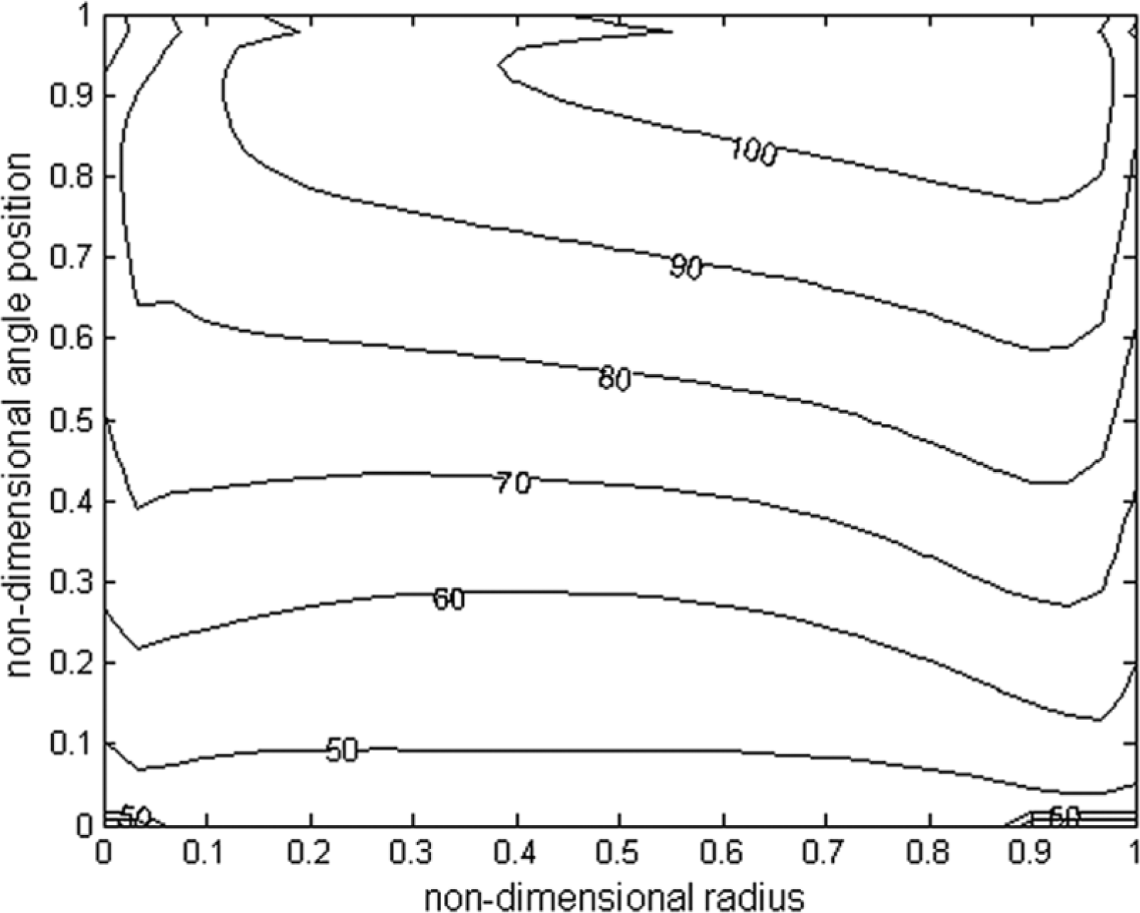
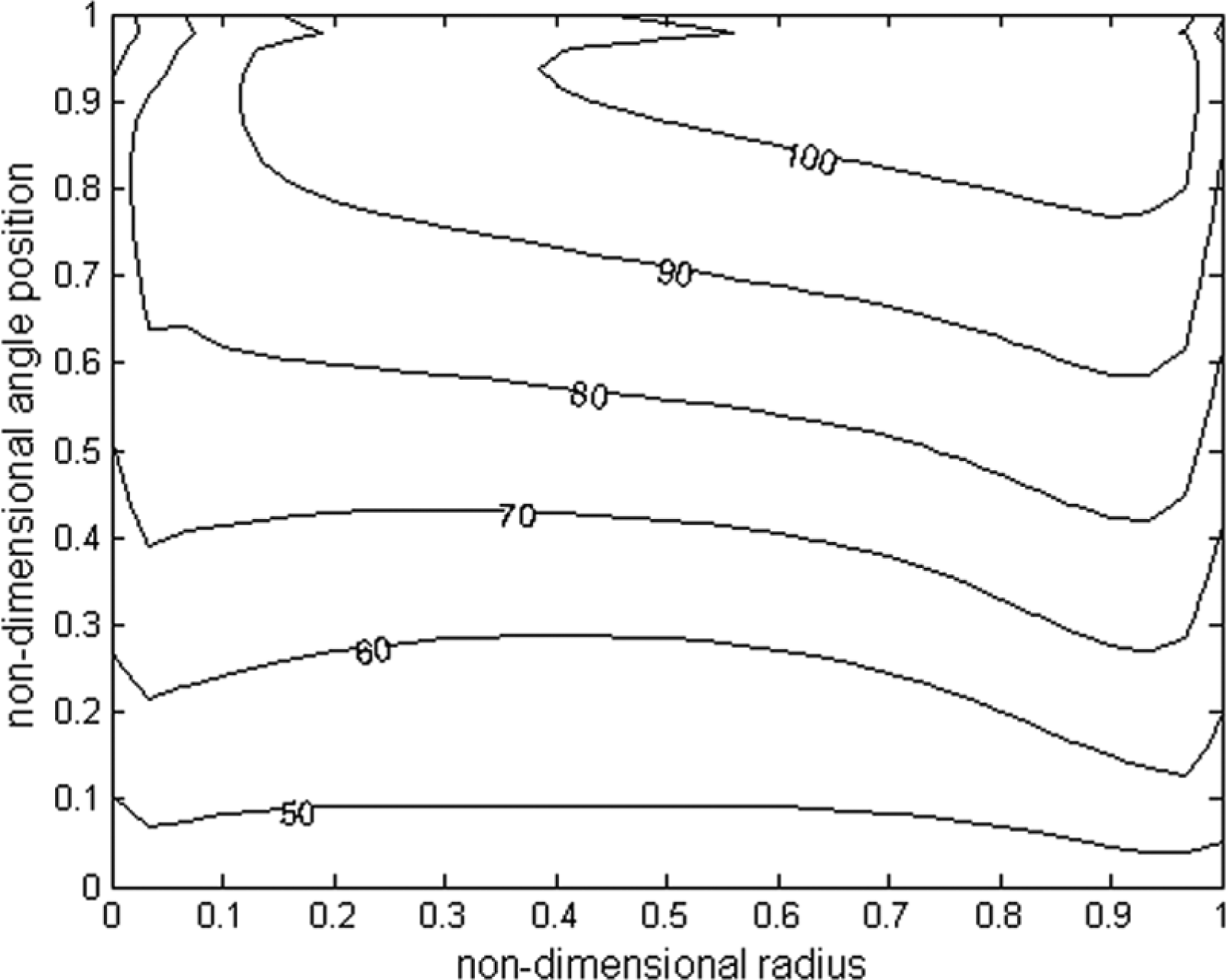
Figures 5 and 6 are the temperature distributions on the film–pad interface of Case 1 obtained from (1) the lubricant film solved by the CBS method and (2) the heat transfer in the bearing pad. These two figures show that the temperature in the lubricant film rises from the leading edge to the tailing edge. The maximum temperature appears at the location where the film thickness is relatively small and the velocity gradient along the z-direction is intense. Figure 7 shows the isothermals at the film–pad interface along the centerline in the direction of the bearing angle. The isothermal of Case 2, which uses the refined mesh resolution, is shown in Figure 8. Little deviation could be found between those two figures, indicating that the original coarser mesh can be used to obtain a mesh-independent solution of the film temperature. The coarser mesh was also used in the analysis done by Wodtke et al., 27 in which the simulation was performed with FDM. This means that the CBS method could obtain steady-state solution of the energy equation with the same mesh density. It is worth to be noted that the vertical axes and the graph in both Figures 7 and 8 are separated by the dashed lines, which indicate the film–pad interface. The lower portions of these axes are non-dimensionalized by referencing the initial film thickness, h 00. The upper portions take B m as the reference value (see Appendix 3 for the expression of B m). In order to show the temperature in a more clear way, in all these figures the unit of the temperature is chosen as °C.
Film temperature profile on film–pad interface: Case 1. The unit of temperature is °C.
Pad temperature profile on film–pad interface: Case 1. The unit of temperature is °C.
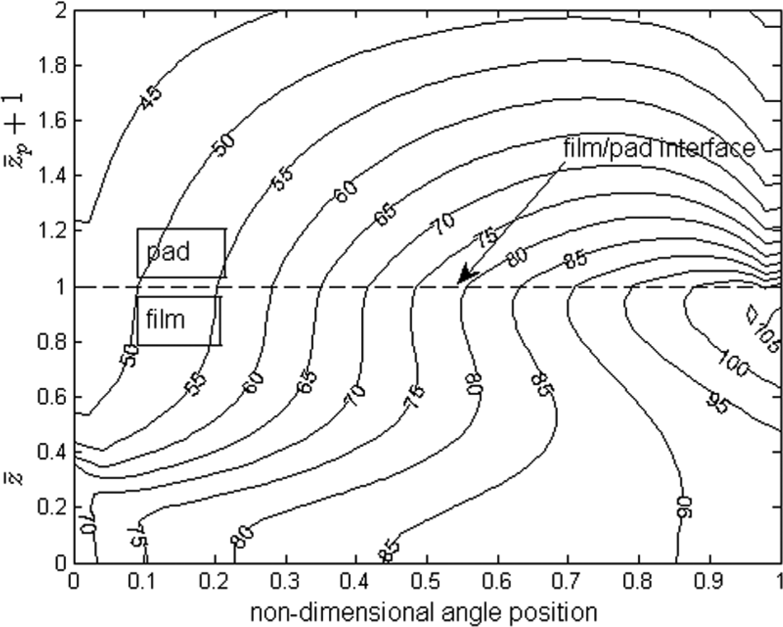
Isothermal between the film and the pad: Case 1. The unit of temperature is °C.

Isothermal between the film and the pad: Case 2. The unit of temperature is °C.
Figure 9 shows the temperature curves along the center of the bearing pad in the circumferential direction on the film–pad interface of Cases 1, 3, and 4. The temperature trends in all these figures are roughly the same. As expected, the more the axial load, the higher the peak temperature. Significant deviation exists when the result of Case 1 is compared with the analysis conducted by Wodtke et al. 27 This may be attributed to the fact that instead of complete TEHD simulation of the tilting-pad thrust bearing, a thermohydrodynamic (THD) analysis of a fixed pad thrust bearing with the same geometry and lubricant property is performed. In this way, the CBS method could be implemented to solve the energy equation without calculating the tilting angle of the bearing pad.

Temperature along the centerline in circumferential direction: Cases 1, 3, and 4. The unit of temperature is °C.
The film temperature solution of Case 5 is illustrated in Figure 10 in the form of isothermal diagram. The lubricant of Case 5 is liquid water, which has much lower viscosity in the temperature range of this study. Water-lubricated thrust bearing usually operates under thinner lubricant film. In this work, the oil film thickness at the center of the bearing pad of Case 1 is about two times the thickness of the water film of Case 5. Case 5 could be a demonstrating simulation of THD analysis with low viscosity lubricant. The result in Figure 10 indicates that the temperature rise across the bearing pad along the centerline in the circumferential direction is about 2.4°C.
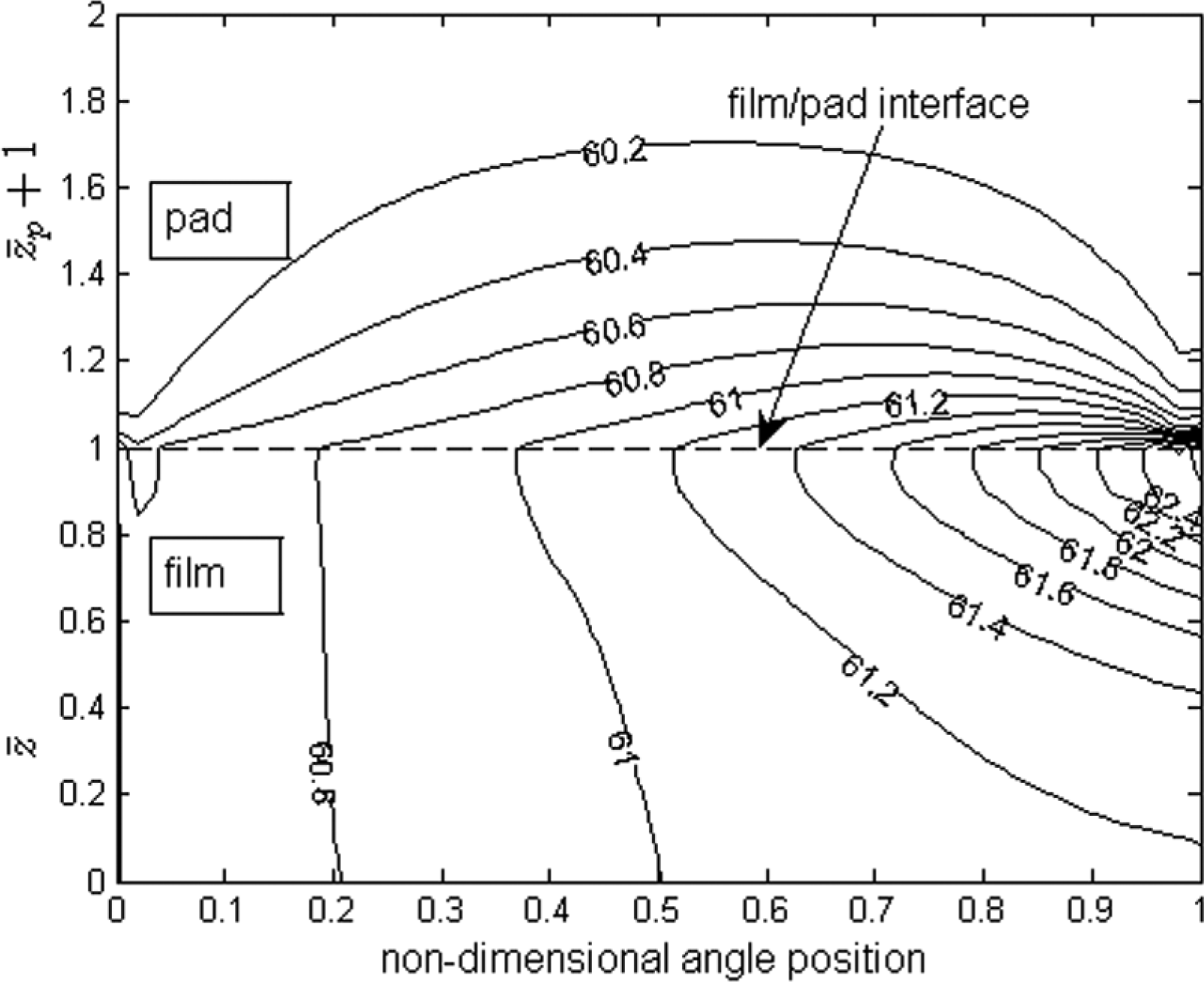
Isothermal between the film and the pad: Case 5. The unit of temperature is °C.
It is observed that the leading edge temperature rises substantially due to the hot oil carry-over effect in Cases 1–4. However, the temperature rise at the leading edge of the water-lubricated thrust bearing under the current simulation settings of this study is negligible.
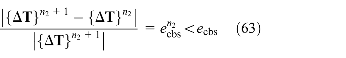
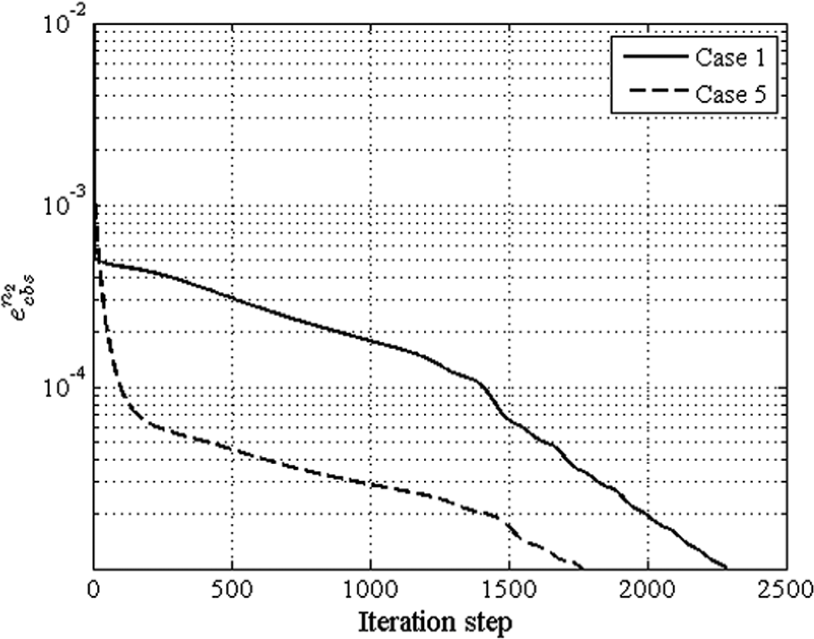
The typical convergence histories of CBS method, equation (60), during the iteration process of Cases 1 and 5 are illustrated in Figure 11. The average time steps needed to achieve the convergence limitation are less than 3000. As shown in Figure 11, when the simulation approximately reaches the steady state, the value expressed by equation (63) is small, making the solution of {
Convergence history of
Although the CBS method and SU/PG method both can be considered as being within the scope of FEM, significant difference can be found between them. SU/PG method mainly deals with the oscillatory solution of convection–diffusion problem by using the PG type of weighting in the FEM formulations. The self-adjointness is achieved by choosing the optimal parameter of the shape functions according to the element’s Peclet number. It is essentially a kind of guesswork. One can easily find out that the mass matrices resulting from SU/PG method are non-symmetric, 9 which will cause difficulty in subsequent solution process. The CBS method, on the other side, obtains its self-adjointness in fundamentally different manner. Consequently, no additional modification or justification is needed on the shape functions.
Conclusion
The energy equation of the analysis of hydrodynamic lubricated thrust bearing is solved by the finite element CBS method. The steady state of the three-dimensional temperature distribution across the lubricant film is obtained in a time-stepping manner.
The results from the case studies show that
The steady-state energy equation, with the convection terms present, can be solved by finite element CBS method.
Steady-state solution can be obtained with similar mesh density compared to FDM.
The CBS method, when used to solve the energy equation, can cope with lubrication with relatively lower lubricant viscosity and thinner lubricant film.
Typical convergence history of the CBS method shows that relatively faster converge behavior could be expected when the steady-state solution is about to be reached.
The CBS method is originally developed to deal with N-S equations. This work has extended its usability in lubrication analysis.
Footnotes
Appendix 1
Appendix 2
Appendix 3
Academic Editor: Noel Brunetiere
Declaration of conflicting interests
The author(s) declared no potential conflicts of interest with respect to the research, authorship, and/or publication of this article.
Funding
The author(s) disclosed receipt of the following financial support for the research, authorship, and/or publication of this article: This work was funded by the National Natural Science Foundation of China (No. 51406114).