Wavelength measurement of a liquid jet based on spectral analysis of image intensity

Abstract

The instability analysis of the liquid jet issuing into ambient gas was conducted with the emphasis placed upon the evolution of surface wave on the jet surface. First, an experimental method was developed to visualize the microscopic surface wave on the liquid jet. Camera setting parameters significantly affecting the detection of desired jet features were discussed. Second, a spectral method was applied to process the obtained jet images. The accuracy of this method was validated in several ways. The results show that wavelengths increase monotonically along the streamwise direction and decrease with the increase in Reynolds number which corresponds to the boundary layer momentum thickness at nozzle exit. Various patterns of wave structures on jet surface are revealed. In this article, the pattern transforms from three-dimensional to two-dimensional at Reynolds number of 134.53.

Introduction

Liquid fuel plays a critical role in most propulsion devices, which considerably elevates the importance of spray formation. According to the environmental conditions, size, distribution, and velocity of droplets are often emphasized in the design of liquid-fuel injectors. In this connection, a proper understanding of spray characteristics is sorely necessary. However, the mechanism of liquid atomization has not been well mastered so far. The study of liquid atomization comprises the evolution of perturbations in the flow in both time and space. But the formation of these perturbations remains a challenging topic. These perturbations will be amplified by the interface force until they become fully developed and result in the generation of droplets. Numerical simulation provides a tool for studying the evolution of these perturbations.^1–4 However, such a tool cannot function without initial and boundary conditions. In most cases, these conditions are deduced with simple theoretical models which cannot explain the physical mechanism involved. The most commonly accepted jet disintegration theories suggest that there exist four different breakup regimes based on the Reynolds and Ohnesorge numbers of the flow.^5,6 These regimes are Rayleigh breakup, first wind-induced breakup, second wind-induced breakup, and atomization. Reported studies about these regimes place their attention on the breakup or spray formation occurring fairly downstream of the nozzle exit. The flow physics near the nozzle exit where initial disturbance takes shape and then develops has not been addressed.

In practice, the jet stream is often featured by appreciably small diameter but high velocity, which leads to various research difficulties. Relevant experimental studies have rarely been reported, and among them, the studies made by Hoyt and Taylor^7,8 and Portillo et al. ⁹ are of significance. Using high-speed photography, Hoyt and Taylor captured turbulent structures on liquid jet surface near the nozzle exit, but wavelength characteristics of these instability waves were not considered in their work. Portillo et al. reproduced Hoyt and Taylor’s work and processed jet images with a power spectrum estimation method, and the latter is recognized as pioneering and significant. Hitherto, no detailed discussion of power spectrum estimation methods has been devoted to the study of liquid jets and the accuracy of image processing was not validated in this aspect.

A new visualization experimental method is presented here, and the determination of the important parameters involved is discussed. Compared with the Welch method which was used in Portillo et al.’s work, the Burg method is used for image processing in this article, and the accuracy of Burg method is validated in several ways. Furthermore, the relationship between jet surface wave and Reynolds number is investigated based on quantitative information extracted from jet images, and the principle illustrating the effect of turbulence on the structure of liquid jet is summarized. This study probes into the physical microscopic scale under which the geometric effect such as surface roughness becomes important. Such a scale is beyond all published studies in this field. The vigorousness of the new method devised here to capture small-scale morphological information is highlighted here and such a method is expected to be extended to other applications.

Experimental approach

Photography techniques

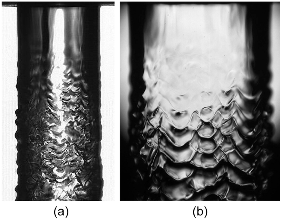
Figure 1(a) is obtained using common photography technique. In appearance, the jet stream is continuous, and the jet stream diameter remains constant for a rather long axial distance. Meanwhile, the interface between liquid jet stream and ambient air is appreciably smooth, and no obvious disturbance near the nozzle exit is detected. There should be traces of disturbance on the interface between the two distinctly different fluids.^10,11 As is evident in Figure 1(b)–(d) that there exits significant complex structures on the interface along the streamwise direction. The difference indicates that conventional photographic method is not capable of capturing the disturbance structures due to insufficient temporal and spatial resolutions.

Figure 1.

Macroscopic and microscopic structures of a liquid jet: (a) the exposure time is 20 ms, and the image resolution is 0.1 mm/pixel; and (b–d) the exposure time is 1 µs, and the image resolution is 0.006 mm/pixel.

Exposure time

The exposure time of the camera must be short enough to capture the jet of high velocity; otherwise, motion blur will take shape, as shown in Figure 2(a). Motion blur is briefly explained in Figure 2(b). The jet is denoted by the solid diamond inside the rectangular windows, and the exposure time ( $\Delta t$ ) is equally divided into three smaller moments ( $(1/3)\Delta t$ ). If the jet moves an appreciable distance during the exposure time, namely, the position of the diamond varies with time. As can be seen in Figure 2(b), the three diamonds will not overlap in the last image, and this is defined as motion blur. In this case, the exposure time should be reduced to $(1/3)\Delta t$ so as to avoid the motion blur. In principle, for continuous motions, exposure time should be infinitely small. However, the distance that the microscope lens can distinguish is limited. Therefore, if the distance covered by the jet during the exposure time is smaller than the distance that the microscope lens can distinguish, the motion can be ignored and motion blur can be avoided accordingly.

Figure 2.

Motion blur: (a) a blurred jet image and (b) schematic diagram of motion blur.

Image resolution

Two jet images with different image resolutions are presented in Figure 3. The two jets are produced under the same experiment condition. But Figure 3(a) is captured by micro-lens, while Figure 3(b) is captured with microscope lens. The image resolution of Figure 3(b) is four times more than that of Figure 3(a). The wave structures can be seen in both images. However, the structures related to Figure 3(b) are more distinct, and more specific information can be obtained. Further research lies heavily on the accuracy of the information. As a note, since the pixel number attached to a camera is limited, the area that the camera can capture will decrease while the image resolution is increased.

Figure 3.

Jet pictures of different image resolutions: (a) 0.0241 mm/pixel and (b) 0.0056 mm/pixel.

Experimental setup

A sketch of the experimental setup and local components near the nozzle are presented in Figure 4. Water flows from a pressurized tank into the nozzle. The jet penetrates through a wooden plate before entering into a container. Mass flow rate is measured by collecting the water discharged into the container and weighting the amount of water collected within a certain period. Water temperature is measured using a WS-T11PRO digital thermometer, so parameters such as density and kinematic viscosity can be obtained thereof. Pressure is measured at the tank and upstream of the nozzle.

Figure 4.

Experimental setup: (a) sketch of the setup and (b) photograph of the setup in the region near the nozzle.

Images are captured using an OLYMPUS I-SPEED 3 high-speed camera equipped with a 12× optical zoom microscope. The amplification of the microscope is set as 2.8, which provides a typical resolution around 0.0056 mm/pixel. Exposure time and frame rate are set as 1 µs and 2000 fps, respectively. The image size of each frame is set to be 1280 × 1024 pixels. The outside diameter of the nozzle and the corresponding pixel value are measured before the experiment. The ratio of the outside diameter of the nozzle to the pixel value serves as an important reference for the calibration (resolution) of the jet images. The light source used in this experiment is OLYMPUS ILP-2. The light beam passes through a 5-mm acrylic diffuser plate before touching the jet surface. The acrylic diffuser plate is used to produce a uniform light distribution. The light, liquid jet, and microscope are colinear.

The schematic diagram of the nozzle used in this study is described in Figure 5. Published articles^7,8 suggest that this kind of nozzle geometry can create a laminar liquid jet. The diameter of the inlet (d) is 8 mm. The overall nozzle geometry consists of a 7.5° half-angle contraction section, followed by a straight section whose inner diameter (D) is 4 mm. Also, the length of the straight section (L) is 4 mm. The contraction section can stabilize the flow, and the gradual transition from contraction section to the straight section can weaken the cavitation effect inside the nozzle.

Figure 5.

Nozzle dimensions.

Experimental results

Flow conditions

The experiment allows variation on Reynolds number ( ${\mathrm{Re}}_{{\delta }_2}$ ) based on the momentum thickness ${\delta }_2$ at the exit of the nozzle. ⁷ The ${\delta }_2$ can be calculated by the laminar Blasius solution for a flat plate

$${\delta }_2=0.664\sqrt{\frac{\nu L}{U}}$$

(1)

where L is the length of the straight section, v is kinematic viscosity, and U is jet velocity.

Substituting ${\delta }_2$ into formula (2) yields the ${\mathrm{Re}}_{{\delta }_2}$ as follows

$${\mathrm{Re}}_{{\delta }_2}=\frac{U{\delta }_2}{\nu }$$

(2)

The calculated flow properties are detailed in Figure 6.

Figure 6.

Experimental flow properties: (a) mass flow rate, (b) velocity, and (c) boundary layer momentum thickness at exit of the nozzle. Reynolds numbers are based on momentum thickness and jet velocity.

Images of jet surface structures

Figure 7 shows the images of surface waves as ${\mathrm{Re}}_{{\delta }_2}$ varies from 96.17 to 111.23. There is no wave structure on the jet surface near the nozzle exit at ${\mathrm{Re}}_{{\delta }_2}=96.17$ . At ${\mathrm{Re}}_{{\delta }_2}=111.23$ , the wave structures similar to fish skin are evidenced on the jet surface. In contrast, smooth jet surface is found near the nozzle exit. With the progression of the jet, the wave structures are stretched in both streamwise and vertical directions. Both the size of those wave structures and the length of the smooth jet segment decrease as ${\mathrm{Re}}_{{\delta }_2}$ increases. At ${\mathrm{Re}}_{{\delta }_2}=134.53$ , “fish skin”-like wave structures almost vanish, and the newly generated two-dimensional wave structures can be found. At ${\mathrm{Re}}_{{\delta }_2}=155.55$ , the surface structures become fully chaotic.

Figure 7.

Evolution of instability waves with the increase in ${\mathrm{Re}}_{{\delta }_2}$ . The x = 0 in every image corresponds to the nozzle outlet section. Y0 indicates the centerline; Yu and Yd are the upper and lower vertical limits, respectively.

Image processing

The wave structures on the jet surface are complex and usually involve multiple scales. Inevitably, some disturbance due to environment will be incorporated into experimentally obtained jet images. In most cases, human eyes cannot distinguish the disturbance on jet images. Therefore, lots of uncertainties will be incurred when observation serves as the major tool in the experiment.

The improvement of data precision necessitates a more feasible image post-processing method. In present experiment, the light beam passes through the liquid jet before hitting the complementary metal oxide semiconductor (CMOS). Thus, the light intensity that photosensitive elements sense differs from the physical jet structure. The photosensitive elements translate light intensities into different image intensities represented by pixels. These pixels serve as the foundation of the jet image. Based on the previous analysis, disturbance structures can be measured using image intensity. As shown in Figure 8(a), a line extends from the nozzle in the streamwise direction. The image intensity distribution along this line is shown in Figure 8(b). As can be observed, the vertical range of 0–471 pixels is associated with fairly weak fluctuation of image intensity, while for the vertical range between 472 and 1023 pixels, the image intensity fluctuations are drastic.

Figure 8.

Image intensities of pixels of a line on the jet image: (a) Image of jet. The x = 0 corresponds to the nozzle outlet section. Y0 indicates the centerline; Yu and Yd are the upper and lower vertical limits, respectively, (b) Image intensity distribution along red line of figure 8(a). Horizontal ordinate corresponding to the sreamwise direction; Longitudinal coordinate represent the image intensities of the pixels along the red line.

In general, the jet stream segment immediately downstream of the nozzle exit is cylindrical, and the wave structures of the jet are not restricted in a single plane. Meanwhile, the depth of field of microscope lens is limited. As a result, if focusing on the plane near the jet axis, the structures of the side region will be indistinct. As can be seen in Figure 7, only the region (x = 0–1.25D, y = Yu − Yd) is distinct. For this region, the minimum pixel length of sampled data should be larger than the size of the surface wave. Therefore, the data length in this article was set as 270 pixels. In Figure 8(b), the distance between the nozzle exit and the position of the first emerged wave structure is 471 pixels. Thus, the midpoint of the first set of data was set at 471, namely, the first set of data was from 337 to 606. Then, the midpoint of data march downstream at an identical step of 80 pixels. For example, the second set of data is collected from 472 to 741. Such a process is then executed in the radial direction.

Comparison of spectral methods for jet image processing

A relevant image processing method has been solely carried out by Portillo et al. ⁹ The method used in their article is the Welch method ¹² which is one of the conventional power spectral methods. The computational formula of the Welch method is expressed as

$$\overline{P}\left(w\right)=\frac{1}{\mathrm{MUL}}\sum _{i=1}^L{\left|\sum _{n=0}^{M-1}{x}_N^i\left(n\right)d\left(n\right)e^{-\mathrm{jwn}}\right|}^2$$

(3)

where N is the number of the data, L is the number of the segments, M is the length of each segment, $x_N^i(n)$ represent one set of the data, $d(n)$ is the window function, $U=(1/M)\sum _{n=0}^{M-1}{d}^2(n)$ is a normalizing factor used to achieve an asymptotic and unbiased estimation, $e^{\mathrm{jwn}}=\cos (\mathrm{wn})+j\sin (\mathrm{wn})$ is the complex sinusoidal, $w$ is the circular frequency, and $\sum _{n=0}^{M-1}{x}_N^i(n)d(n)e^{-\mathrm{jwn}}$ is the Fourier transform of random sequence of segment $i(1\le i\le L)$ .

According to the principle of the Welch method, the result of the Welch method depends heavily on the selection of window function $d(n)$ . The window function used in Portillo et al.’s article is Blackman window which has less sideband leakage but wider main lobe, which indicates that the resolution of Blackman window is not sufficient. Unfortunately, there is still no any other window function that can improve both resolution and variance of power spectrum estimation.

Instead of the Welch method, the method used in this article is the Burg method, which is one of the modern power spectrum estimation methods. The Burg method does not require window function. The computational formula of the Burg method is

$$P_x\left(e^{\mathrm{jw}}\right)=\frac{{\sigma }^2}{{|1+\sum _{k=1}^p{a}_k{e}^{-\mathrm{jwk}}|}^2}$$

(4)

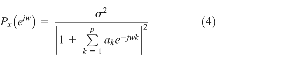
where $p$ is the degree of model, $k=1,2,\dots ,p$ , ${\sigma }^2$ is the variance of white noise, and $a_k$ is the coefficient. The $a_k$ and $p$ can be calculated by the Yule–Walker equation. ¹³

One set of data of Figure 8(a) is taken up for processing with the Welch method and the Burg method separately. The results are shown in Figure 9. The abscissa of the biggest wave crest is the wavelength. The wavelengths of the two methods are the same. But the Burg method has larger energy ratio of the main lobes to the first side lobe, that is to say, the Burg method can well mitigate the disturbance of the side lobe. Meanwhile, the width of the main lobe of the Burg method is much smaller than that of the Welch method, which means that the resolution of the Burg method is much better. With respect to the jet image processing discussed here, the Burg method is better than the Welch method.

Figure 9.

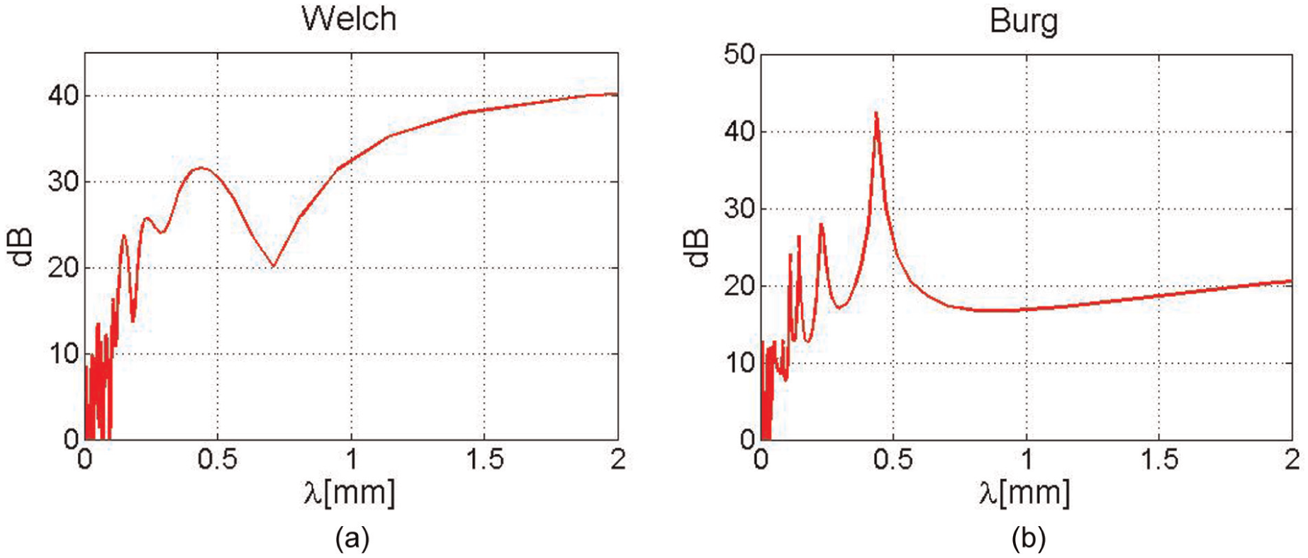
Comparison of (a) the Welch method and (b) the Burg method.

Validation of the Burg method

In this section, the accuracy of the Burg method is validated with both a periodical integer sequence and a periodic object. Also, the Burg method is used to process the jet images of Portillo et al.’s article and compare with the results reported in their article.

First, an array which has a fixed cycle and length is used to validate the accuracy of the Burg method. The array is as follows

$$\mathrm{A}=\{0,1,2,3,4,0,1,2,3,4\dots \}$$

The wavelength (cycle) of the array is 5. The length of the array is 270, same as the length of the data extracted from Figure 8.

This array is processed by the Burg method, and the results are shown in Figure 10. The obtained wavelength of the maximum crest is 5, which is in well accordance with the actual value.

Figure 10.

Power spectrum curve of a group of deterministic signals.

The signals that we need to process come from the jet images. Analogously, the signals which get from a ruler image are used for processing in the second validation method.

Figure 11(a) is an image of a ruler. The value of one scale of the ruler is 1 mm, and the corresponding pixel length is 87 pixels. The Burg method is used to process the signals that come from ruler image. The result is shown in Figure 11(b). The wavelength of the maximum crest of the curve is 85.33 pixels. The error is only 1.9%. The error may come from the noise that is introduced by the scratch, spot, and nonuniform illumination. But even under this condition, the Burg method still has a good effect.

Figure 11.

Validation with a ruler image: (a) image of a ruler and (b) result of the Burg method.

Furthermore, the jet images in Portillo et al.’s paper were also processed with the Burg method. The results are shown in Figure 12. The wavelengths we obtained are from a single image, and the jet image resolution that comes from Portillo et al.’s article is different from that reported. With these in mind, the two results are consistent with each other.

Figure 12.

Wavelengths (solid) obtained by the Burg method applied to jet images from Portillo et al. ⁹ versus data from reference (hollow).

Discussion

The results of wavelength measurements with the Burg method along the streamwise direction are illustrated in Figure 13. After obtaining a measured λ at a streamwise position, the process is repeated for all the other available spanwise positions, and the average value of these wavelengths is represented by $\overline{\lambda }$ . The process is repeated for all the 100 images under the same flow condition, and $\overline{\overline{\lambda }}$ is defined as the mean value over 100 images.

Figure 13.

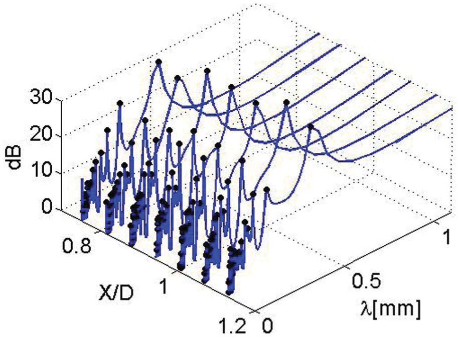
Power spectral density distributions with the Burg method. Each curve represents a specific streamwise location. Circles denote the local maxima of each curve. The wavelength at a specific location corresponds to the global maximum of each curve.

The wavelength distributions at different ${\mathrm{Re}}_{{\delta }_2}$ values along the streamwise direction are presented in Figure 14. The results show that (1) the wavelengths increase monotonically along the streamwise direction. With the liquid jet emanating from the nozzle, the boundary condition for the jet stream will change from no-slip boundary condition to free surface boundary condition. The relaxation of the velocity profile is one of the reasons for the increase in wavelength. ¹⁴ A positive streamwise strain rate which is generated by the flow accelerates on the jet surface near the nozzle exit is another reason for the increase in wavelength. ⁹ (2) The wavelength decreases with the increase in ${\mathrm{Re}}_{{\delta }_2}$ . According to relevant theories, ¹⁵ the wavelengths can be scaled by the momentum thickness. Also, the momentum thickness of the boundary layer becomes smaller as ${\mathrm{Re}}_{{\delta }_2}$ increases. (3) The position that the wave structure initially takes shape approaches the nozzle exit as ${\mathrm{Re}}_{{\delta }_2}$ increases. Wave patterns are produced at the location where the flow transitions from absolutely unstable flow (AU) to convectively unstable flow (CU). ¹⁶ Our data show that this position shifts toward the nozzle exit as Reynolds number increases.

Figure 14.

Wavelength measurements at various streamwise locations.

According to the analysis by Yoon and Heister ¹⁷ and Brennen, ¹⁸ the predicted wavelength can be obtained from

$$\lambda =\frac{2\pi }{{\omega }_r}\left[\frac{U_w}{U_J}\right]{\delta }_2$$

(5)

where ${\omega }_r=0.177$ is the most unstable nondimensional frequency, $U_w$ is the wave velocity, and $U_J$ is the centerline velocity of the liquid jet.

The predicted wavelengths based on the assumption that the wave velocity is close to jet velocity are plotted in Figure 15. As we can see the experimental data from several Reynolds numbers at various streamwise locations almost collapse to a curve that shares a similar variation trend given by Yoon and Heister’s prediction. Portillo and Blaisdell ¹⁴ overprediction of wavelength may rise from a neglected fact that wave velocity varies along the streamwise direction and is not constantly equal to the centerline jet velocity.

Figure 15.

Comparison of wavelength. The heavy line denotes the predicted wavelengths under the assumption that wave velocity is close to jet velocity.

Conclusion

A visualization method that used to capture the micro surface wave is proposed. Primary parameters of this visualization method are discussed. The principles of the Welch method and the Burg method are analyzed, and the Burg method was used for image processing. Several methods are designed to validate the accuracy of the Burg method. The wavelengths of different Reynolds numbers at various streamwise locations were measured and compared with the predicted wavelengths. The main conclusions are as follows:

1. The high temporal and spatial resolutions should be provided to capture the high speed and microstructures. The exposure time must be shorter than the ratio of lens’ appreciable distance to jet velocity. Meanwhile, the microscope with appropriate amplification factor should be used to provide sufficient resolution which is less than the microstructure of the jet. The Burg method can provide accurate result that does not depend on window functions.

2. The wavelengths increase along the streamwise direction, which is partly attributed to the relaxation of the velocity profile and positive streamwise strain rate. The increase in turbulence intensity results in the decrease in wavelength.

3. Diverse wave patterns are found on the surface of the liquid jet. At ${\mathrm{Re}}_{{\delta }_2}=111.23$ , only three-dimensional pattern wave structures are manifested on the jet surface. The wave pattern almost translates into two-dimensional at ${\mathrm{Re}}_{{\delta }_2}=134.53$ .