Sage Journals: Discover world-class research

Abstract

The traditional bearing fault diagnosis method is achieved often by sampling the bearing vibration data under the Shannon sampling theorem. Then, the information of the bearing state can be extracted from the vibration data, which will be used in fault diagnosis. A long-term and continuous monitoring needs to sample and store large amounts of raw vibration signals, which will burden the data storage and transmission greatly. For this problem, a new bearing fault diagnosis method based on compressed sensing is presented, which just needs to sample and store a small amount of compressed observation data and uses these data directly to achieve the fault diagnosis. First, several over-complete dictionaries are trained by dictionary learning method using the historical operating data of the bearings. Each of these dictionaries can be effective in signal sparse decomposition for a particular state, while the signals corresponding to other states cannot be decomposed sparsely. According to this difference, the bearing states can be identified finally. The fault diagnosis results of the proposed method with different parameters are analyzed. The effectiveness of the method is validated by experimental tests.

Keywords

Compressed sensing bearing fault diagnosis dictionary learning signal representation error

Introduction

Considering the material defects, manufacturing errors, working conditions, and other factors such as fatigue, aging, and so on, the damages and faults of the rotating machinery occur inevitably during operation. The bearing is one of the most common and most important key components in rotating machinery; in case of failure, this will lead to the equipment downtime which affects productivity and results in economic loss. Thus, it is particularly important for rotating machinery to execute bearing condition monitoring and fault diagnosing.

The traditional fault diagnosis method is achieved often by sampling the bearing vibration data under the Shannon sampling theorem. The long-term and continuous monitoring needs to sample and store large amounts of raw vibration signal, which will burden the data storage and transmission greatly. The compressed sensing theory can provide a new idea in solving this problem. In 2006, Candès proved in mathematic principle that the original signal could be reconstructed using parts of its Fourier transform coefficients, which would be the theoretical foundation for compressed sensing.¹ Then, Donoho² and Candès³ proposed the concept of compressed sensing formally based on the related work. The main process of compressed sensing can be divided into two steps. First, combining the sampling with the compressing, we can acquire the nonadaptive linear projections (or measurements) of the original signal. Then, the original signal can be reconstructed directly with these measurements by the appropriate recovery algorithms.^4–7 With this strategy, the amount of data in monitoring will be reduced greatly, and the burden in data transmission and storage will be alleviated effectively. Since it is possible to recover the original high-dimensional signal from the compressed measurements with low dimension, which means that most of the bearing state information is contained in these low-dimensional measurements,^8–12 then we can consider achieving the bearing fault diagnosis just using the compressed measurements directly, without recovering the original signal. This is the starting point of our proposed method.

The other sections of this article are organized as follows: in section “Compressed sensing theory,” we will briefly introduce the basic theory of the compressed sensing; the theory of the proposed bearing fault diagnosis method using the compressed measurements directly will be presented in section “Fault diagnosis method”; in section “Experimental test,” the proposed method will be tested with different bearing vibration signals; and, finally, in section “Conclusion,” this article will be summarized.

Compressed sensing theory

For a signal $x \in R^{N}$ , in the frame of compressed sampling, we should get the linear projections of signal x first, which can be converted into an observation matrix $Φ \in R^{M \times N}$ , where each row of the matrix $Φ$ can be regarded as a sensor that multiplies with the signal, and parts of information of the signal will be acquired. Carrying out the compressive measuring to x as

y = Φ x

(1)

Then, we can acquire the compressed measurements (or observations) $y \in R^{M}$ . If x can be recovered from y, which means that these fewer observations contain enough information to recover signal x, then the compressed sensing can be achieved. According to the linear algebra theory, when M is less than N, then equation (1) should have infinitely many solutions and we cannot recover the original signal x uniquely from the low-dimensional signal y. However, if x is sparse, meaning that there is only a few nonzero coefficients in x, then the number of the unknowns will decline greatly, which make it possible to recover x from y.

Actually, the signal x is not sparse in general, but it can be represented sparsely using proper ways such as orthogonal transformation. If we expand $x \in R^{N}$ on some orthogonal basis ${ψ_{i}}_{i = 1}^{N}$ , where $ψ_{i}$ is an N-dimensional column vector, then the signal x can be represented as

x = \sum_{i = 1}^{N} θ_{i} ψ_{i}

(2)

where $θ_{i} = 〈 x, ψ_{i} 〉 = ψ_{i}^{T} x$ is defined as the expansion coefficient. Equation (2) can be transferred into a matrix form as

x = Ψ θ

(3)

where $Ψ = [ψ_{1}, ψ_{2}, \dots, ψ_{N}] \in R^{N \times N}$ is defined as a dictionary matrix with orthogonal basis, and $θ = [θ_{1}, θ_{2}, \dots, θ_{N}]^{T}$ is the expansion coefficient vector. Suppose that the coefficient vector $θ$ is K-sparse on dictionary matrix $Ψ$ , meaning that there is K nonzero elements in $θ$ and K is less than N, then the vector $θ$ can be entitled as sparse representation coefficient of x on dictionary matrix $Ψ$ . Substituting equation (3) into equation (1) and denoting $A^{CS}$ as $Φ Ψ$ , then we can get

y = Φ Ψ θ = A^{CS} θ

(4)

The compressed measurements can be represented in matrix form as Figure 1. Owing to the fact that the vector $θ$ is sparse, then the number of the unknowns in equation (4) will be reduced greatly, so that it is possible to recover $θ$ from y. In order to reconstruct the sparse vector $θ$ , Candès and Tao^6,13 presented and also proved that the $A^{CS}$ mentioned above must satisfy restricted isometry property (RIP) and then Baraniuk¹⁴ proposed the idea that the irrelevance between the observation matrix $Φ$ with the dictionary matrix $Ψ$ was the equivalent conditions of RIP. In case that these conditions satisfied, then we can reconstruct sparse representation coefficient vector $θ$ according to equation (4). After the vector $θ$ being obtained, the original signal x can be easily recovered based on equation (3). There have been many kinds of algorithms to achieve the signal reconstruction, specifically given in previous works^15–25 in detail. The matching pursuit (MP) algorithm will be used to reconstruct signals in this article.¹⁵

Figure 1.

Matrix form of the compressed measurements.

In the previous introduction, the original signal x is represented sparsely on the dictionary with orthogonal basis. However, this kind of dictionary has limited capacity to the signal sparse representation. Therefore, other types of the dictionaries such as a variety of over-complete dictionaries are often used in practice. According to the difference in the applications, over-complete dictionaries can be divided into two categories: fixed dictionaries which can be used for nonspecific signals and trained dictionaries which can be used only for specific signals. In general, the fixed dictionary can be used for many different kinds of signals, but it is difficult to decompose the signal very sparsely, and the signal representation error would be larger. While the trained dictionary can decompose the signal very sparsely since the structure and characteristics information of the training samples is used in dictionary learning process; therefore, the signal sparse representation result can be very good. However, this kind of dictionaries can be used only for the signals which have the same state with the training samples. The most frequently used dictionary learning methods are the method of optimal directions (MODs)^26,27 and the K-singular value decomposition (K-SVD) method.^28,29 In this article, the over-complete dictionaries corresponding to different bearing states will be trained by the K-SVD method.

Fault diagnosis method

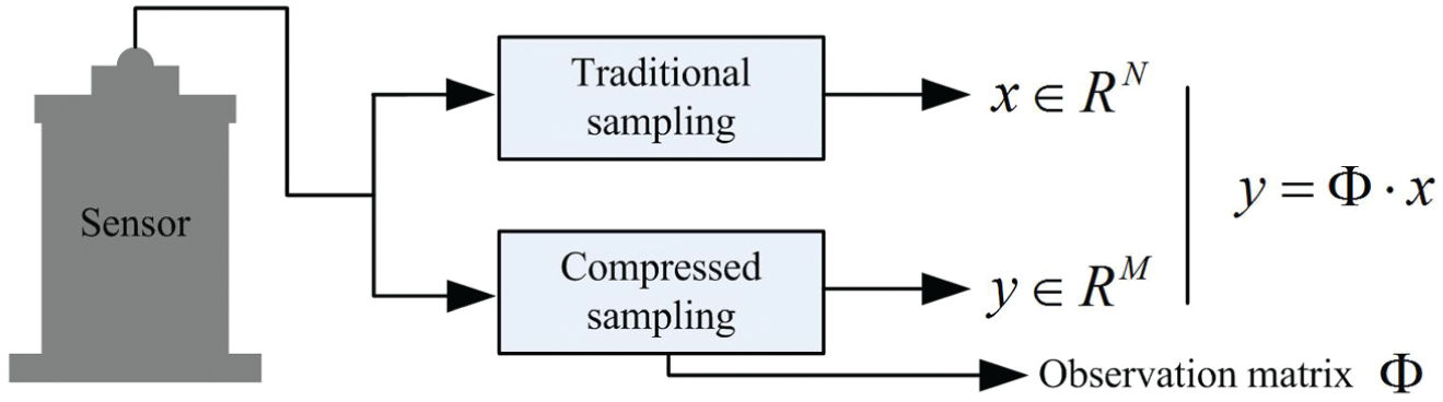
For the acquisition of the bearing vibration signal, we denote the collected high-dimensional signal by $x \in R^{N}$ based on the traditional Nyquist sampling theorem, while the low-dimensional compressed signal is denoted by $y \in R^{M}$ based on the compressed sampling theory. According to the compressed sensing theory, a high-dimensional signal x should correspond to a one-to-one low-dimensional signal y (shown in Figure 2). If we denote the observation matrix corresponding to the compressed sampling way by $Φ \in R^{M \times N}$ , then we can obtain $y = Φ \cdot x$ .

Figure 2.

Relationship between the traditional sampling and compressed sampling.

We define $D_{0}$ as the over-complete dictionary trained with the historical operating data of the bearing in a normal state and $D_{i}$ (i = 1, 2, …, n) as the over-complete dictionary trained with the signals in fault state i. Each of these dictionaries is only available to the signals which have the same state with the corresponding training samples, meaning that the signals in other states cannot be decomposed sparsely on this dictionary. Expanding the high-dimensional signal x on the dictionaries $D_{i}$ (i = 0, 1, 2, …, n) as

x = D_{i} \cdot c_{i}, i = 0, 1, 2, \dots, n

(5)

where $c_{i}$ is the expansion coefficient vector of signal x on dictionary $D_{i}$ . According to the relation between x and y as $y = Φ \cdot x$ , we can obtain

y = Φ \cdot D_{i} \cdot c_{i}, i = 0, 1, 2, \dots, n

(6)

Defining ${\tilde{c}}_{i}$ as the estimate of the expansion coefficient vector $c_{i}$ , then the representation errors of the low-dimensional compressed signal on dictionary $D_{i}$ (i = 0, 1, 2, …, n) can be solved as

δ_{i} = ‖ y - Φ \cdot D_{i} \cdot {\tilde{c}}_{i} ‖_{2}, i = 0, 1, 2, \dots, n

(7)

Then, we can obtain n + 1 representation errors as $δ_{0}, δ_{1}, δ_{2}, \dots, δ_{n}$ .

For a low-dimensional compressed signal y, the representation errors $δ_{0}, δ_{1}, δ_{2}, \dots, δ_{n}$ corresponding to the dictionaries $D_{0}$ , $D_{1}$ , $D_{2}$ , …, $D_{n}$ , respectively, can be calculated. When the compressed signal y is sampled from the bearing in the normal state, then it can be represented sparsely only on the dictionary $D_{0}$ with the representation error as $δ_{0}$ . According to the characters of the dictionary by training, the error $δ_{0}$ would be the smallest one of all the representation errors, namely, $δ_{0} = min {δ_{0}, δ_{1}, δ_{2}, \dots, δ_{n}}$ . Meantime, the error $δ_{0}$ should be smaller. Ideally, it should be close to zero. Similarly, when the compressed signal y is sampled from the bearing in fault state p, $p \in {1, 2, \dots, n}$ , then it can be represented sparsely only on the dictionary $D_{p}$ with the representation error as $δ_{p}$ . In this case, the error $δ_{p}$ would be the smallest one of all the representation errors, namely, $δ_{p} = min {δ_{0}, δ_{1}, δ_{2}, \dots, δ_{n}}$ . Ideally, $δ_{p}$ should be close to zero.

According to the above analysis, the bearing states can be identified by comparing the representation errors of the low-dimensional compressed signal on different dictionaries. The process of the proposed fault diagnosis method is shown in Figure 3, and the corresponding steps are as follows:

Acquiring the high-dimensional vibration signals when the bearing works in different states, which will be used as the training samples in dictionary learning;

Training the over-complete dictionaries ( $D_{0}$ , $D_{1}$ , $D_{2}$ , …, $D_{n}$ ) corresponding to the normal state, fault state 1, fault state 2, …, and fault state n, respectively, with some appropriate dictionary learning methods;

Setting the thresholds ( $τ_{0}$ , $τ_{1}$ , $τ_{2}$ , …, $τ_{n}$ ) of the signal representation errors corresponding to the bearing in the normal state, fault state 1, fault state 2, …, and fault state n, respectively, according to the prior knowledge;

Acquiring the low-dimensional vibration signals $y \in R^{M}$ by compressed sampling. Taking $Φ \in R^{M \times N}$ as the observation matrix, then the high-dimensional signal corresponding to low-dimensional signal y can be denoted by $x \in R^{N}$ and $y = Φ \cdot x$ ;

Representing the low-dimensional signal y on all the known dictionaries ( $D_{0}$ , $D_{1}$ , $D_{2}$ , …, $D_{n}$ ), respectively, and calculating the corresponding representation errors as $δ_{i} = ‖ y - Φ \cdot D_{i} \cdot {\tilde{c}}_{i} ‖_{2}, i = 0, 1, 2, \dots, n$ , where ${\tilde{c}}_{i}$ is the estimate of the expansion coefficient vectors of signal y on matrix $Φ D_{i}$ . Finding the smallest one of these errors as $δ$ , namely, $δ = min {δ_{0}, δ_{1}, δ_{2}, \dots, δ_{n}}$ ;

Estimating the state of the bearing:

When $δ = δ_{0}$ and $δ \leq τ_{0}$ , then the bearing is determined in the normal state;

When $δ = δ_{i}$ and $δ \leq τ_{i}$ , $i \in {1, 2, \dots, n}$ , then the bearing is determined in fault state i;

When $δ$ cannot satisfy any one of the above terms, then we determine the bearing in some unknown state.

Figure 3.

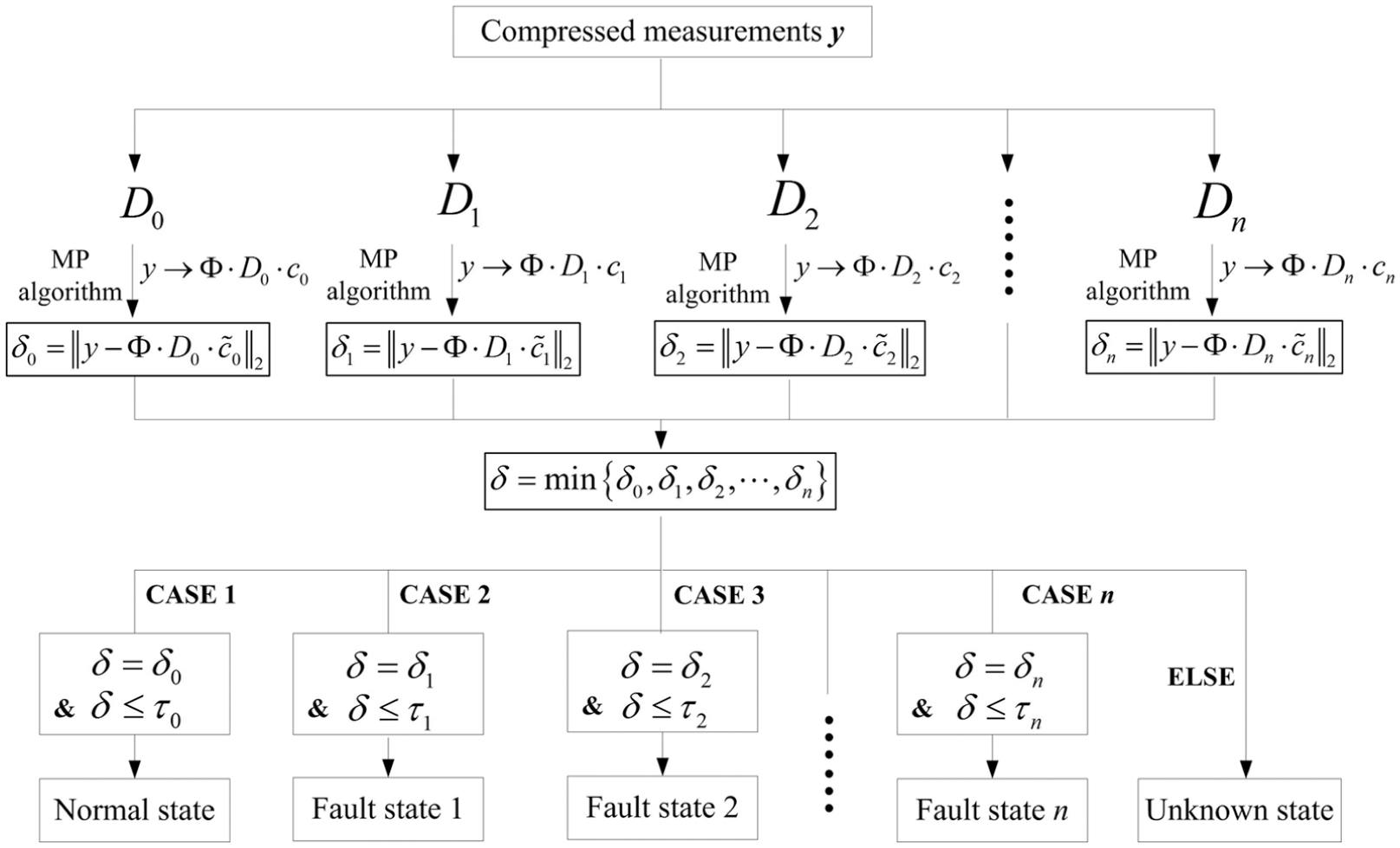
Flowchart of the proposed bearing fault diagnosis method.

In the diagnostic process shown in Figure 3, we determine that the bearing is in some unknown state and confirm that the bearing is in the fault state but not a known fault state. Actually, if more samples corresponding to different fault states can be acquired, then we can obtain more dictionaries by training, which can be used to recognize the unknown bearing state. The dictionaries corresponding to different states play a role similar to a sieve, which can filter the signals with the corresponding state and achieve the identification of the bearing state ultimately. For the error thresholds corresponding to different states, they can be set according to the prior knowledge.

The reason why we set different thresholds of signal representation errors is that there have been many different types of bearing faults, and we cannot obtain enough dictionaries by training to describe all the possible bearing states. For some signal which is not in any one of the known states, if we decompose this signal on all the known dictionaries ( $D_{0}$ , $D_{1}$ , $D_{2}$ , …, $D_{n}$ ), then we can consequentially find the minimum value in all the corresponding signal representation errors ( $δ_{0}$ , $δ_{1}$ , $δ_{2}$ , …, $δ_{n}$ ). If we do not restrict this value and determine the bearing state according to this value directly, then the signal state must be judged as the one of the n + 1 known states (the normal state, fault state 1, fault state 2, …, and fault state n). However, according to the foregoing assumption, this signal does not belong to any one of the above-described states, which will result in a misjudgment to the type of the bearing fault. Therefore, we introduce the thresholds ( $τ_{0}$ , $τ_{1}$ , $τ_{2}$ , …, $τ_{n}$ ) of the signal representation errors to restrict the minimum value, that is, the bearing state can be determined only when both of the following conditions are satisfied:

The error $δ$ is the smallest one of all the signal representation errors;

The error $δ$ should not be greater than the corresponding threshold of the signal representation errors.

As can be seen from the fault diagnosing process, the proposed method is mainly affected by the following factors: the principle to determine the fault state, the signal reconstruction algorithm, and the compressed sampling way. The signal reconstruction algorithm is used to solve the expansion coefficient vector $\tilde{c}$ , and the MP algorithm will be used in this article. Accordingly, the main parameters which affect the fault diagnosing results include the threshold of the signal representation error, the sparsity set in MP algorithm, the amount (M) of the compressed measurements, and the type of the observation matrix $Φ$ . In the next section, the impacts of these parameters on the bearing fault diagnosis will be analyzed.

Experimental test

The proposed fault diagnosing method is validated using the vibration signals from the 6205-2RS JEK SKF deep groove ball bearings (data sources are from Case Western Reserve University Bearing Data Center Website,³⁰ and the signal sampling frequency is 12K). The data used in our tests can be divided into two types: the training samples used in dictionary learning and the test samples used for the validation of the proposed method. The signals sampled in a traditional way should be high-dimensional. For dictionary learning, the high-dimensional samples can be used directly. While the test samples should be low-dimensional, in our tests, they will be obtained by simulating the compressed sampling. 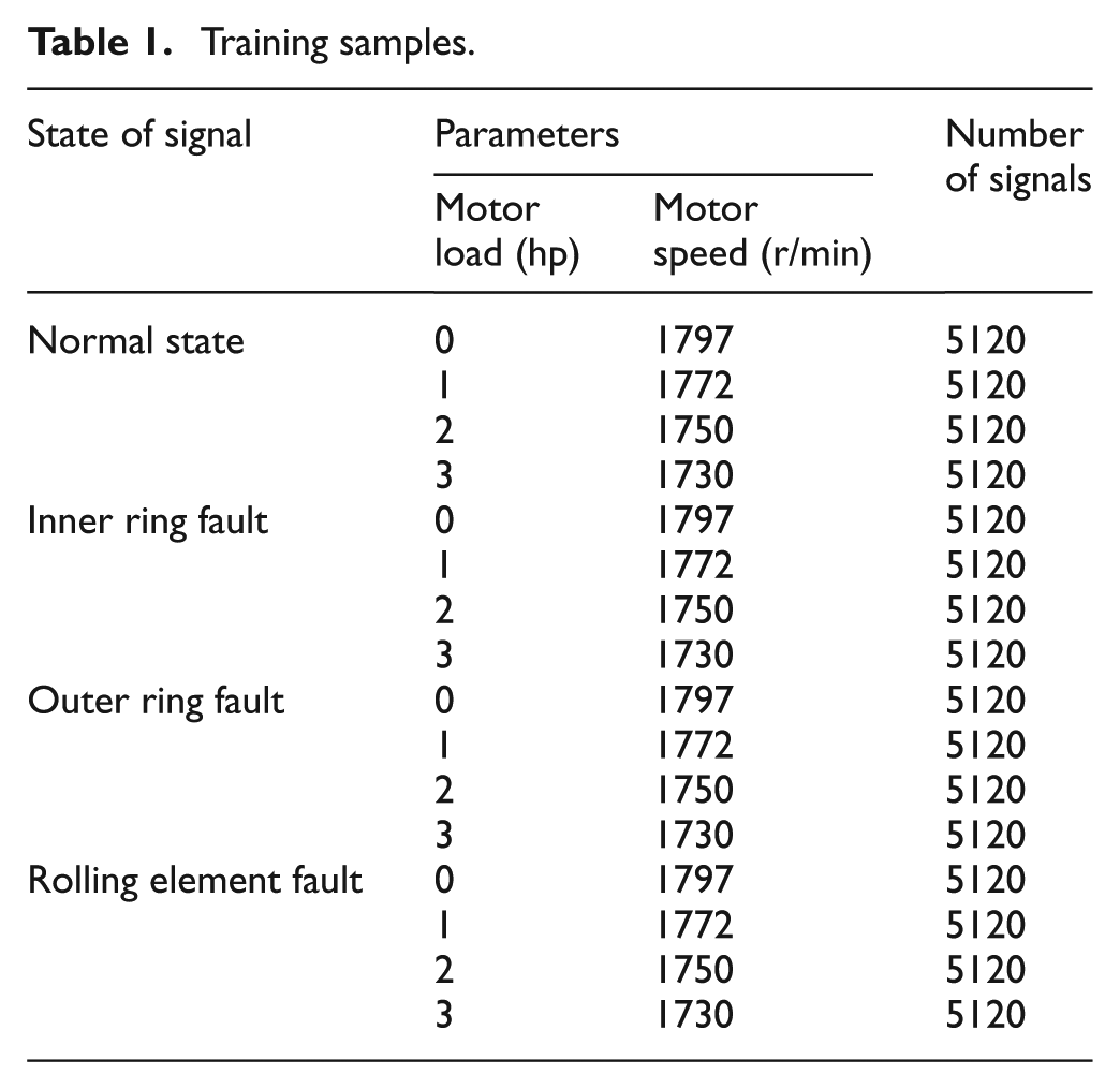Defining $Φ \in R^{M \times N}$ as the observation matrix, then each high-dimensional signal has N data points, and each low-dimensional signal has M data points. In our tests, we set N as 512.

The training samples can be divided into four categories: normal state samples, inner ring fault samples, outer ring fault samples, and rolling element fault samples. Each type of the samples contains 20,480 signals, which can be also divided into four groups, and each group contains 5120 signals according to different motor speeds and loads. The training samples are shown in Table 1.

Table 1.

Training samples.

State of signal	Parameters		Number of signals
State of signal	Motor load (hp)	Motor speed (r/min)	Number of signals
Normal state	0	1797	5120
	1	1772	5120
	2	1750	5120
	3	1730	5120
Inner ring fault	0	1797	5120
	1	1772	5120
	2	1750	5120
	3	1730	5120
Outer ring fault	0	1797	5120
	1	1772	5120
	2	1750	5120
	3	1730	5120
Rolling element fault	0	1797	5120
	1	1772	5120
	2	1750	5120
	3	1730	5120

Then, the over-complete dictionaries ( $D_{normal}$ , $D_{inner}$ , $D_{outer}$ , and $D_{ball}$ ) corresponding to the normal state, inner ring fault, outer ring fault, and rolling element fault can be trained, respectively, by K-SVD dictionary learning method using the above training samples. The parameters in dictionary learning are set as follows: the quantity of atoms is set to 1024, the sparsity is set to 10, the number of loops is set to 20, and the initial dictionary is selected from the training samples.

The original high-dimensional test samples contain 800 signals corresponding to the normal state and 1200 signals corresponding to the fault states. The fault can be divided into three categories: the inner ring fault, outer ring fault, and rolling element fault. For each type of fault, we acquire 400 signals. Considering that the effects of variable speed operation or variable loads are extremely common in industrial applications, we will analyze the data with different levels of speed and motor load in our experimental tests. In accordance with different motor speeds and loads, the test samples corresponding to each bearing state contain four groups of signals, as shown in Table 2. The faults were designed as single point in inner ring, outer ring, and rolling elements, which were introduced to the test bearings using electrodischarge machining with fault diameter of 0.021 in and fault depth of 0.011 in.

Table 2.

Original high-dimensional test samples.

State of signal	Parameters		Number of signals
State of signal	Motor load (hp)	Motor speed (r/min)	Number of signals
Normal state	0	1797	200
	1	1772	200
	2	1750	200
	3	1730	200
Inner ring fault	0	1797	100
	1	1772	100
	2	1750	100
	3	1730	100
Outer ring fault	0	1797	100
	1	1772	100
	2	1750	100
	3	1730	100
Rolling element fault	0	1797	100
	1	1772	100
	2	1750	100
	3	1730	100

In order to set appropriate error thresholds, we will refer to the prior knowledge. For each bearing state, we can select some training samples randomly in Table 1, taking 1000 signals, for instance, and then the corresponding low-dimensional signals can be obtained by simulating the compressed sampling. Denoting the observation matrix by $Φ \in R^{M \times N}$ , then the simulation can be achieved by carrying out the compressive measuring to x as $y = Φ \cdot x$ , where $x \in R^{N}$ is the high-dimensional signal in Table 1, and $y \in R^{M}$ (M < N) is the corresponding low-dimensional signal. The Gaussian random matrix¹⁴ is taken as the compressed observation matrix, and the amount (M) of the measurements is set as 80. The signal representation errors of these low-dimensional compressed signals on different dictionaries can be calculated, respectively, where the sparsity in MP algorithm is set as 10. The results are shown in Figure 4. Figure 4(a) shows the representation errors of the signals in the normal state on the four dictionaries ( $D_{normal}$ , $D_{inner}$ , $D_{outer}$ , and $D_{ball}$ ), respectively. Figure 4(b) shows the representation errors of the inner ring fault signals on the four dictionaries, respectively. Figure 4(c) shows the representation errors of the outer ring fault signals on the four dictionaries, respectively. Figure 4(d) shows the representation errors of the rolling element fault signals on the four dictionaries, respectively. The data in each figure can be divided into two parts. The circles indicate the representation errors of the signals on the dictionary corresponding to the same state with the current signals. The points in the figure describe the representation errors of the signals on other dictionaries.

Figure 4.

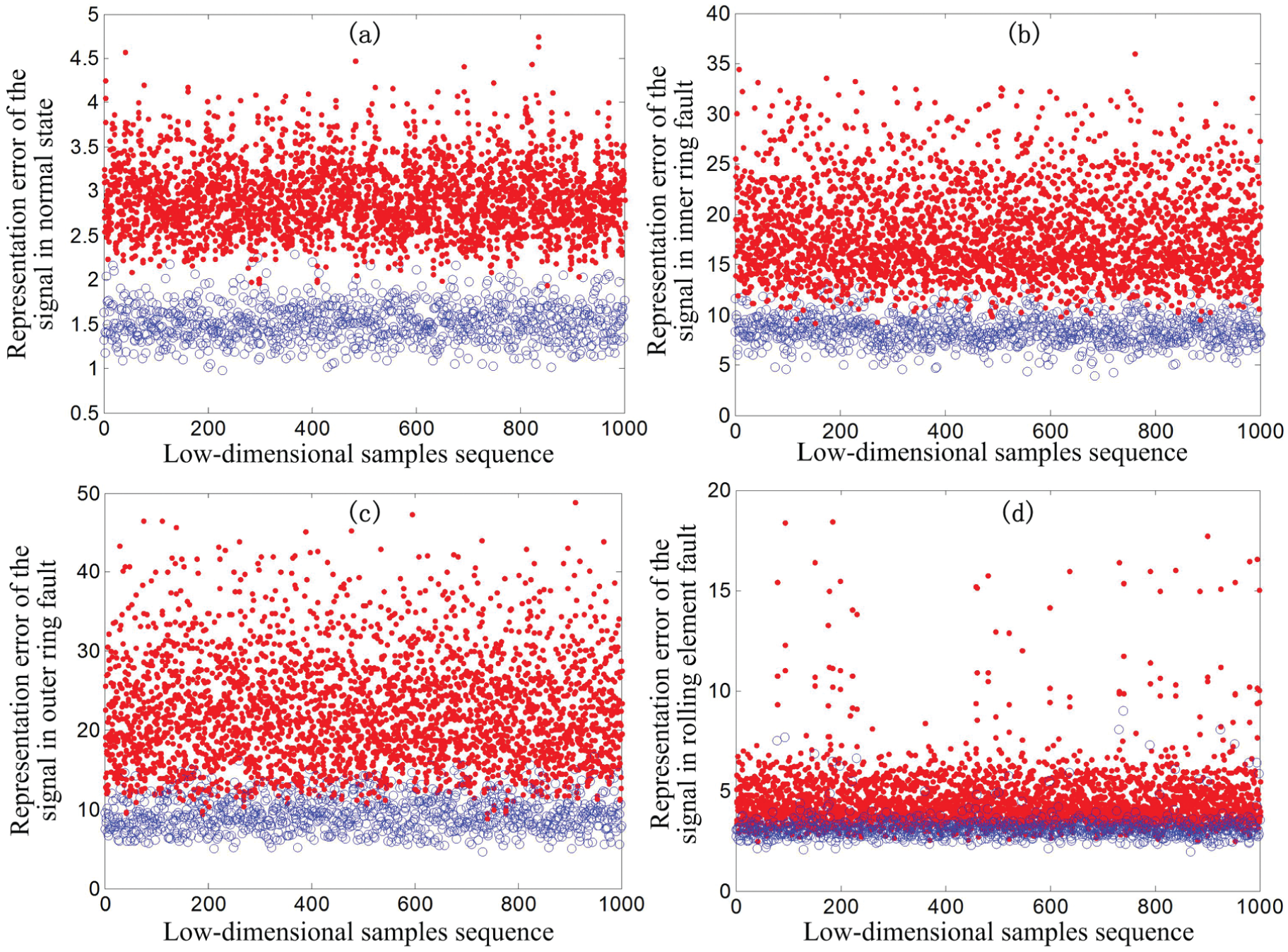
Representation errors of the low-dimensional signals on different dictionaries: (a) normal state, (b) inner ring fault, (c) outer ring fault, and (d) rolling element fault.

Ideally, the two parts of the data in Figure 4 should be separated completely according to the principle of the proposed fault diagnosis method. This means that for each state, the corresponding error threshold should be more than all of the values indicated by the circles and less than all of the values indicated by the points. Actually, this ideal case is extremely difficult to achieve in practice. Therefore, the following principle will be used in setting the thresholds: for each state, the corresponding error threshold should be more than most of the values indicated by the circles and less than most of the values indicated by the points in the corresponding figure. In all of our tests, we will follow the “95% principle,” meaning that the threshold will be set as the value which is more than and just more than 95% representation errors of the signals. For example, for the error threshold corresponding to the normal state, we can set it as the value which is more than and just more than 950 data indicated by the circles in Figure 4(a). Defining $τ_{normal}$ , $τ_{inner}$ , $τ_{outer}$ , and $τ_{ball}$ as the error thresholds corresponding to the normal state, inner ring fault, outer ring fault, and rolling elements fault, respectively, these thresholds can be set as 2.0, 11.2, 13.4, and 3.9, respectively according to the above principle.

Taking Gaussian random matrix¹⁴ as the observation matrix in compressed sampling and setting the amount (M) of the compressed measurements as 80, then we can obtain the low-dimensional signals corresponding to the original test samples as shown in Table 2. As mentioned in our article, in order to reconstruct the sparse representation vector, the observation matrix should be irrelevant to the dictionary used in signal sparse representation. In our tests, the dictionaries are always trained with different training samples, meaning that these dictionaries are not constant and can be changed when the training samples change. Due to the fact that Gaussian random matrix can be irrelevant to most of the transform matrices, it can be used as the compressed observation matrix in most of the cases. That is why we take Gaussian random matrix as the compressed observation matrix in our tests.

In our proposed method, the bearing states can be determined just using these low-dimensional signals directly. The expansion coefficient vector is solved by the MP algorithm, where the sparsity of the coefficient vector is set as 10. Then, the bearing fault diagnosing can be achieved, and the results are shown in Table 3. The recognition rate to some state characterizes the ratio of the amount of the samples identified accurately to the amount of all the test samples in this state. It can be seen from Table 3 that the recognition rates of the proposed method to the normal state reach to 97.88%, and for the fault states, the recognition rates can be up to 80%. Meanwhile, the low-dimensional signals which cannot be identified correctly are determined to be in some unknown state. These results validate the effectiveness of the proposed method to the bearing fault diagnosing.

Table 3.

Fault diagnosing results.

State of signals	Actual amount	Recognized amount	Recognition rate (%)
Normal state	800	783	97.88
Inner ring fault	400	324	81
Outer ring fault	400	341	85.25
Rolling element fault	400	321	80.25

According to the theory and process of the fault diagnosing used above, the thresholds of the signal representation errors have a significant impact on the diagnosing results. Keeping other parameters invariable, Figure 5 shows the recognition rates of the four bearing states when the corresponding error thresholds change. Figure 5(a) shows the recognition rates of the normal state when the error threshold $τ_{normal}$ changes. Figure 5(b) shows the recognition rates of the inner ring fault when the error threshold $τ_{in}$ changes. Figure 5(c) shows the recognition rates of the outer ring fault when the error threshold $τ_{out}$ changes. Figure 5(d) shows the recognition rates of the rolling element fault when the error threshold $τ_{ball}$ changes.

Figure 5.

Recognition rates of the bearing states with different error thresholds: (a) normal state, (b) inner ring fault, (c) outer ring fault, and (d) rolling element fault.

It can be seen from Figure 5 that with the increase in the error thresholds, the recognition rates of the four bearing states will increase gradually. However, it should be noted that the thresholds should not be very large, although a larger threshold can improve the recognition rate of the corresponding state. A very large threshold will increase the possibility of misjudging when the signal is actually in some unknown state. In next test, we take the 400 signals corresponding to the outer ring fault as shown in Table 2 as the original high-dimensional test samples. Taking Gaussian random matrix as the observation matrix in compressed sampling and setting the amount (M) of the compressed measurements as 80, then we can obtain the low-dimensional signals corresponding to these original test samples. Suppose we obtain only three over-complete dictionaries as $D_{normal}$ , $D_{inner}$ , and $D_{ball}$ by training, then the desired results should be that all of these 400 test samples are determined to be in some unknown states according to the proposed method; otherwise, the results should be incorrect.

The expansion coefficient vector is solved by the MP algorithm, where the sparsity of the coefficient vector is set as 10. If we keep the threshold $τ_{normal}$ as 2.0 and $τ_{ball}$ as 3.9, then the misjudging rates can be calculated when the threshold $τ_{in}$ changes. The misjudging rate is defined as the ratio of the amount of the misjudged samples to the total number of the test samples. Then, the fault diagnosing results are shown in Figure 6.

Figure 6.

Misjudging rates of the bearing state with different error thresholds $τ_{in}$ .

It can be seen from Figure 6 that with the increase in the error threshold $τ_{in}$ , the misjudging rate will increase gradually (in fact, most of the misjudged samples are determined to be in the inner ring fault), which would be a disadvantage to the fault diagnosing. Therefore, we should make full use of the prior knowledge to set the thresholds of the signal representation errors appropriately, namely, not too small or too large.

In the above tests, the sparsity set in MP algorithm was set as 10 all the time, meaning that the number of the atoms involved in the representation of the low-dimensional signals is kept 10. According to the fault diagnosis theory in this article, the number of the atoms used in signal representation affects the sparse representation errors directly. Then, the fault diagnosing results will also be affected. Similar to the previous tests, we keep the thresholds of signal representation errors as follows: the threshold $τ_{normal}$ is set as 2.0, the threshold $τ_{inner}$ is set as 11.2, the threshold $τ_{outer}$ is set as 13.4, and the threshold $τ_{ball}$ is set as 3.9. The recognition rates of the different states are calculated with different sparsities in MP algorithm, and the results are shown in Figure 7.

Figure 7.

Recognition rates of the different states with different sparsities in MP algorithm.

As can be seen from Figure 7, with the increase in the sparsity, the recognition rates of the normal state, inner ring fault, and outer ring fault will gradually improve, while the recognition rates of the rolling element fault show a trend of increasing first and then declining slightly. In general, a larger sparsity in MP algorithm is of benefit to bearing fault diagnosing. This result should relate to the character of the dictionaries. Taking the dictionary corresponding to the normal state for example, with the increase in the sparsity, the atoms involved in signal representation will increase. In this case, the signals in the normal state can be represented more accurately, and the corresponding representation errors will become smaller. While this dictionary is not available for the signals in other states, therefore, with the sparsity increasing, the corresponding representation errors cannot improve significantly. According to the fault diagnosis theory of the proposed method, this difference in representation errors will be of benefit to the state identification. That is why the state recognition rates improved with the increasing sparsity. For the trend that the recognition rates of the rolling element fault declined when the sparsity becomes larger, the following analysis may be taken as an explanation. For the dictionary corresponding to the rolling element fault, with the increase in the sparsity, not only the representation errors of the signals in the rolling element fault on this dictionary decline but also the representation errors of the signals in other states decline. In this case, the difference in the representation errors corresponding to different states will shrink, which may result in the declining of the recognition rates.

Although a larger sparsity in MP algorithm is propitious to the bearing state identification, we must note that the sparsity should not be very large, for a too large sparsity will bring in the increasing of the computation, which should be a disadvantage to bearing fault diagnosing. Therefore, we should set the sparsity as a moderate size. In general, the sparsity in MP algorithm can be set as the value which is equal to the sparsity set in dictionary learning, just as what we did in this article.

In the previous analysis, we just used 80 compressed measurements in fault diagnosing. The following analysis will focus on the bearing fault diagnosis with different amount of the compressed measurements. The error thresholds will always be set by the “95% principle” introduced above. In this test, the Gaussian random matrix is taken as the observation matrix. The expansion coefficient vector is solved by MP algorithm, and the sparsity of the coefficient vector is set as 10. Then, the recognition rates of the four states with different amount (M) of the compressed measurements are calculated, and the results are shown in Figure 8.

Figure 8.

Recognition rates of the four states with different amount (M) of the compressed measurements.

It can be seen from Figure 8 that when M is less than 100, with the increase in the compressed measurements, the recognition rates of the four states will improve first and then being stabilized gradually on the whole, which means that more compressed measurements is of benefit to the bearing fault diagnosing. The more the compressed measurements, the more the information of the bearing operation will be contained, which is propitious to the bearing state identification. The less compressed measurements will alleviate the burden of the data storage and transmission, which is also a disadvantage to the fault diagnosing in the meantime. The more compressed measurements will be an advantage to the fault diagnosing, but the effectiveness in alleviating the burden of the data storage and transmission will be weaken accordingly. In practice, we should give full consideration to both of the two factors and set a moderate amount of the compressed measurements.

In the experimental tests of this section, we obtained the compressed measurements by taking the Gaussian random matrix as the observation matrix. Actually, different compressed sampling systems will correspond to different observation matrices, and of course, we can also use other compressed sampling ways. To validate our proposed method with different compressed sampling ways, we will analyze and compare the fault diagnosing results in several typical compressed sampling ways (based on Gaussian random matrix,¹⁴ partial orthogonal matrix,⁶ and Toeplitz and circulant matrices,³¹ respectively). The error thresholds will always be set by the “95% principle” introduced above. The expansion coefficient vector is solved by MP algorithm, and the sparsity is set as 10. Then, the recognition rates of the four bearing states when using different observation matrices are calculated, respectively, and the results are shown in Figure 9. Figure 9(a) shows the recognition rates of the normal state in the three compressed sampling ways. Similarly, Figure 9(b)–(d) shows the recognition rates of the inner ring fault, outer ring fault, and rolling element fault, respectively.

Figure 9.

Fault diagnosing results corresponding to different observation matrices: (a) normal state, (b) inner ring fault, (c) outer ring fault, and (d) rolling element fault.

As can be seen from Figure 9, when M is less than 100, with the increase in the compressed measurements, the recognition rates of the four bearing states will show an overall trend of improving gradually and then being stabilized in all of the three compressed sampling ways. This means that more compressed measurements are of benefit to the fault diagnosing in most cases, no matter which compressed sampling way we use. This results show that the proposed method is effective when taking any one of the three compressed sampling ways. The results in Figure 9 also indicate that the fault diagnosing result when using Toeplitz and circulant matrices is slightly better than that when using other two observation matrices. The fluctuations of the recognition rates in each figure should be attributed to the randomness introduced when building the observation matrix and setting the thresholds.

Conclusion

A bearing fault diagnosis method based on the low-dimensional compressed measurements is proposed in this article. In the proposed method, it is not necessary to reconstruct the original high-dimensional signals. The bearing fault diagnosis can be achieved using a small amount of compressed measurements directly and then the data we need to acquire for diagnosing can be reduced greatly, which will alleviate the burden in data storing and transmission. The main parameters which affect the fault diagnosing results include the threshold of signal representation error, the sparsity set in MP algorithm, the amount of the compressed measurements, and the type of the observation matrix. The impacts of these parameters on the fault diagnosing results are analyzed, respectively, in this article, and some conclusions can be summarized as follows:

The error thresholds in the proposed method can be set by referring to the prior knowledge;

The sparsity in MP algorithm can be set as the value which is equal to the sparsity set in dictionary learning;

More compressed measurements are propitious to the state identification;

The Toeplitz and circulant matrices in compressed sampling has better performance in fault diagnosing.

Footnotes

Acknowledgements

The authors gratefully acknowledge the Bearing Data Center of Case Western Reserve University for providing the bearing test data. Valuable comments on this article from anonymous reviewers are very much appreciated.

Academic Editor: Fakher Chaari

Declaration of conflicting interests

The authors declare that there is no conflict of interest.

Funding

This study was financially supported by National Natural Science Foundation of China under grant nos 51375484, 51205401, and 51475463.

References

Candés

Romberg

Tao

. Robust uncertainty principles: exact signal reconstruction from highly incomplete frequency information. IEEE Trans Inform Theor 2006; 52: 489–509.

Donoho

. Compressed sensing. IEEE Trans Inform Theor 2006; 52: 1289–1306.

Candès

. Compressive sampling. In: Proceedings of international congress of mathematicians, Madrid, 22–30 August 2006, pp.1433–1452. Switzerland: European Mathematical Society Publishing House.

Candès

Wakin

. An introduction to compressive sampling. IEEE Signal Process Mag 2008; 25: 21–30.

Donoho

Tsaig

. Extensions of compressed sensing. Signal Process 2006; 86: 533–548.

Candès

Tao

. Near optimal signal recovery from random projections: universal encoding strategies. IEEE Trans Inform Theor 2006; 52: 5406–5425.

Davenport

Boufounos

Wakin

. Signal processing with compressive measurements. IEEE J Sel Top Signal Process 2010; 4: 445–446.

Duarte

Davenport

Wakin

. Sparse signal detection from incoherent projections. In: Proceedings of the IEEE international conference on acoustics, speech and signal processing (ICASSP), Toulouse, 14–19 May 2006, pp.305–308. New York: IEEE.

Duarte

Davenport

Wakin . Multiscale random projections for compressive classification. In: Proceedings of the IEEE international conference on image processing (ICIP), San Antonio, TX, 16 September–19 October 2007, pp.161–164. New York: IEEE.

10.

Haupt

Castro

Nowak

. Compressive sampling for signal classification. In: Proceedings of the asilomar conference on signals, systems and computers, Pacific Grove, CA, 29 October–1 November 2006, pp.1430–1434. New York: IEEE.

11.

Haupt

Nowak

. Compressive sampling for signal detection. In: Proceedings of the IEEE international conference on acoustics, speech and signal processing (ICASSP), vol. 3, Honolulu, HI, 15–20 April 2007, pp.1509–1512. New York: IEEE.

12.

Davenport

Wakin

Baraniuk

. Detection and estimation with compressive measurements. Technical report TREE0610, 2006. Houston, TX: Department of Electrical and Computer Engineering, Rice University.

13.

Candès

Tao

. Decoding by linear programming. IEEE Trans Inform Theor 2005; 51: 4203–4215.

14.

Baraniuk

. A lecture on compressive sensing. IEEE Signal Process Mag 2007; 24: 118–121.

15.

Mallat

Zhang

. Matching pursuit with time-frequency dictionaries. IEEE Trans Signal Process 1993; 41: 3397–3415.

16.

Friedman

Tukey

. A projection pursuit algorithm for exploratory data analysis. IEEE Trans Comput 1974; 23: 881–890.

17.

Mallat

Davis

Zhang

. Adaptive time-frequency decompositions. Opt Eng 1994; 33: 2183–2191.

18.

DeVore

Temlyakov

. Some remarks on greedy algorithms. Adv Comput Math 1996; 5: 173–187.

19.

Blumensath

Davies

. Stagewise weak gradient pursuit. IEEE Trans Signal Process 2009; 57: 4333–4346.

20.

Needell

Vershynin

. Uniform uncertainty principle and signal recovery via regularized orthogonal matching pursuit. Found Comput Math 2008; 9: 317–334.

21.

Blumensath

Davies

. Gradient pursuit. IEEE Trans Signal Process 2008; 56: 2370–2382.

22.

Davis

Mallat

Avellaneda

. Adaptive greedy approximations. Constr Approx 1997; 13: 57–98.

23.

Chen

Donoho

Saunders

. Atomic decomposition by basis pursuit. SIAM Rev 2001; 43: 129–159.

24.

Chen

Donoho

Saunders

. Atomic decomposition by basis pursuit. SIAM J Sci Comput 1999; 20: 33–61.

25.

Fuchs

. On sparse representations in arbitrary redundant bases. IEEE Trans Inform Theor 2004; 50: 1341–1344.

26.

Engan

Aase

Husoy

. Multi-frame compression: theory and design. Signal Process 2000; 80: 2121–2140.

27.

Engan

Aase

Hakon-Husoy

. Method of optimal directions for frame design. In: Proceedings of the IEEE international conference on acoustics, speech, and signal processing (ICASSP), vol. 5, Phoenix, AZ, 15–19 March 1999, pp.2443–2446. New York: IEEE.

28.

Aharon

Elad

Bruckstein

. K-SVD: an algorithm for designing of overcomplete dictionaries for sparse representation. IEEE Trans Signal Process 2006; 54: 4311–4322.

29.

Aharon

Elad

Bruckstein

. On the uniqueness of over-complete dictionaries, and a practical way to retrieve them. Linear Algebra Appl 2006; 416: 48–67.

30.

http://csegroups.case.edu/bearingdatacenter/pages/download-data-file

31.

Yin

Morgan

Yang

. Practical compressive sensing with Toeplitz and circulant matrices. Technical report TR10-01, 2010. Houston, TX: Department of Computational and Applied Mathematics (CAAM), Rice University.

A bearing fault diagnosis method based on the low-dimensional compressed vibration signal

Abstract

Keywords

Introduction

Compressed sensing theory

Fault diagnosis method

Experimental test

Conclusion

Footnotes

Acknowledgements

Declaration of conflicting interests

Funding

References